
*Photo by Steshka Willems from Pexels*
Introduction to the Introduction
So, this definitely got out of hand. Started out by thinking I’d do a simple, little correlation analysis, which then ended up as a dive into transformed variables for linear regression, which also entailed some outlier analysis, which then turned into an exploration into ggplot and diagnostic plots, and then also using kable() to produce tables in RMarkdown. All code is available on my GitHub.
Introduction
I was recently reading a piece on Baseball Prospectus discussing defensive metrics in baseball that left me with a few questions. While I do think it is a great breakdown of the current defensive metrics, something I’ve been curious about since first looking at the defensive rankings on the back of Strat-O-Matic cards, I was left a bit bothered by the line, “defensive quality is nowhere near as important as hitting or pitching, but it is important nonetheless.” My issue with this is that it strikes me as biased. Not for explicitly stating that offense and pitching are more important than defense, but because offensive and pitching metrics are more readily available and robust than defensive metrics. It may be that offense and pitching appear more contributory because they are more measures and they are more easily measured. It reminds me of how when I studied behavioural psychology we were effectively told that internal mechanisms like thoughts were not considered because they could not be measured accurately through the (at-the-time) current standards of assessment. Furthermore, as important for what? Wins? Losses? Runs? Outs?
Going with these questions, I decided to do a basic correlation analysis between wins, losses, runs scored, runs allowed, and runs allowed minus home runs allowed. This was to examine whether the number of runs allowed or runs scored, as stand-ins for defensive performance and offensive performance respectively, had a stronger correlation with wins or losses. These are very basic stand-ins, and I wouldn’t recommend using them beyond a cursory analysis of a team’s performance.
In addition to the correlation analysis I also did a linear regression analysis to see which of runs scored or runs allowed would better account for the variance in the opposing dependent variable (i.e., runs scored and losses and runs allowed and wins). Results for the correlation analysis and linear regression models as well as limitations and future directions are discussed below.
Side note: I want to re-iterate that these analyses are very basic and do not go into as much depth as would be needed to properly explore the topics discussed in this post. However, they do provide a basis from which, at least I think, to begin understanding the contributions of offence and defence in baseball, as well as how our understanding or perception of a thing is influenced by the way in which we measure or assess it.
Data & Methods
All data for this analysis comes from the Lahman R package Teams dataset. For this analysis, I only used games from 1961 onward as that is when the 162 game season was introduced. This left 1566 observations. I also only used the columns yearID (year of season), W (number of wins), L (number of losses), R (number of runs scored), RA (number of runs allowed), and HRA (number of home runs allowed). The reason for including home runs allowed was to subtract that from runs allowed as a makeshift calculation for removing pitcher influence from runs allowed. However, given that not all home runs are solo home runs this is not a perfect substitute.
Missing Values
The data was examined for the presence of missing values and none were found (huzzah!).
Correlation Analysis
Looking at Table 1 for correlation results, it can be seen that runs scored had a 0.59 correlation with wins, while runs allowed had a -0.31 correlation with wins (also see Figure 1 for a visualization). Meaning that runs scored and wins were more closely associated with each other than runs allowed and wins. Additionally, runs scored had a -0.27 correlation with losses, while runs allowed had a correlation of 0.62 (see Table 1 and Figure 1). Meaning that runs allowed and losses were more closely associated with each other than runs scored and losses. Regarding the removal of home runs from runs allowed, the correlation results increased with runs allowed minus home runs allowed (RA_MHRA) returning a correlation of 0.66 with losses and -0.37 with wins (see Table 1 and Figure 1).
| W | L | R | RA | RA_MHRA | |
|---|---|---|---|---|---|
| W | 1.00 | -0.30 | 0.69 | 0.00 | -0.02 |
| L | -0.30 | 1.00 | 0.04 | 0.72 | 0.75 |
| R | 0.69 | 0.04 | 1.00 | 0.60 | 0.52 |
| RA | 0.00 | 0.72 | 0.60 | 1.00 | 0.96 |
| RA_MHRA | -0.02 | 0.75 | 0.52 | 0.96 | 1.00 |
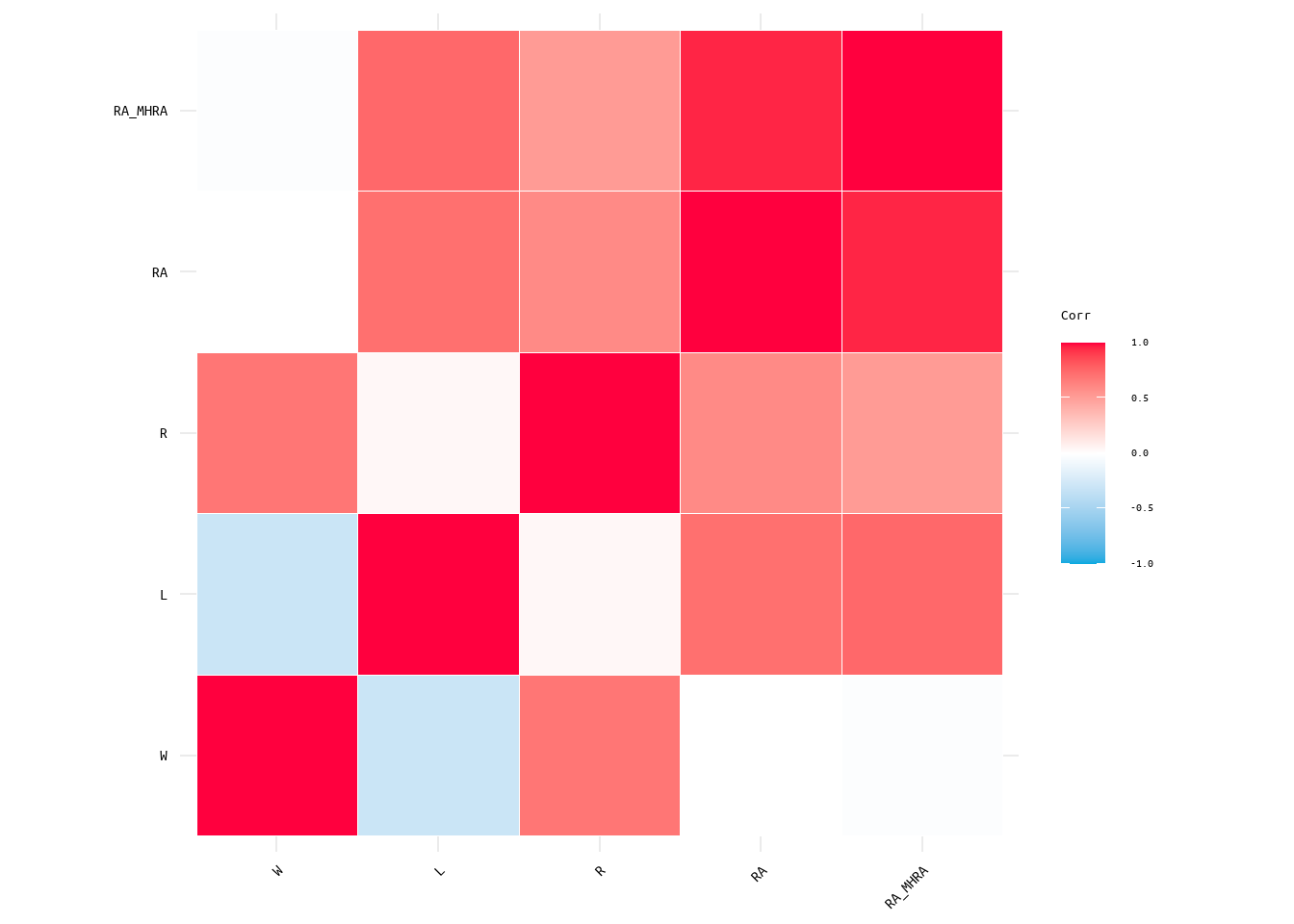
Figure 1: Heatmap Correlation Matrix for Wins, Losses, Runs, Runs Allowed, and Runs Allowed Minus Home Runs
Regression Analysis
In addition to the correlation analysis, a linear regression analysis was also performed for each of wins and losses with runs scored, runs allowed, and runs allowed minus home runs allowed. The purpose being to see which of runs scored or runs allowed contributed more to the variance in the associated correlation variable (i.e., runs scored to wins and runs allowed to losses), but also to see which of runs scored or runs allowed contributed more to the variance in the opposing variable (i.e., runs scored to losses and runs allowed to wins).
Data Summary
To gain a better understanding of the data and possible influences on the models, a summary of the data with the min/max values, quartiles, and median and mean values was generated. Results can be seen in Table 2. Additionally, a histogram was generated for each variable to better understand the distribution (see Figure 2).
Looking at Table 2 and Figure 2, the variables appear to have a fairly Gaussian distribution. Although, some values in the extremes may cause issues for model performance.
| W | L | R | RA | RA_MHRA | |
|---|---|---|---|---|---|
| Min. : 19.00 | Min. : 17.00 | Min. : 219.0 | Min. : 209.0 | Min. :141.0 | |
| 1st Qu.: 71.00 | 1st Qu.: 71.00 | 1st Qu.: 640.0 | 1st Qu.: 638.0 | 1st Qu.:503.0 | |
| Median : 80.00 | Median : 79.00 | Median : 703.0 | Median : 700.0 | Median :556.0 | |
| Mean : 78.86 | Mean : 78.86 | Mean : 697.1 | Mean : 697.1 | Mean :550.3 | |
| 3rd Qu.: 89.00 | 3rd Qu.: 88.00 | 3rd Qu.: 767.2 | 3rd Qu.: 769.0 | 3rd Qu.:608.0 | |
| Max. :116.00 | Max. :120.00 | Max. :1009.0 | Max. :1103.0 | Max. :862.0 |
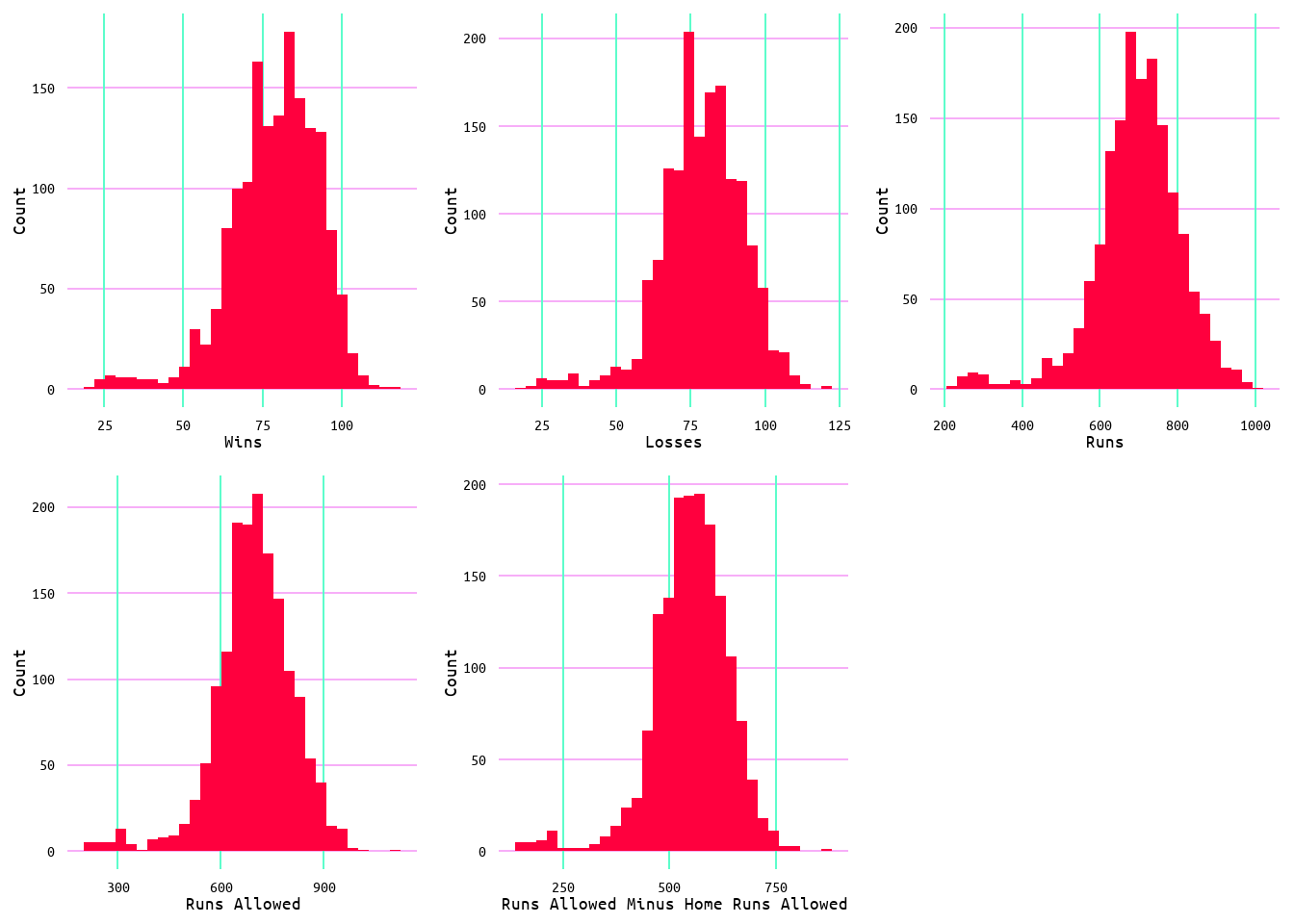
Figure 2: Distribution of Variables Wins, Losses, Runs Scored, Runs Allowed, and Runs Allowed Minus Home Runs Allowed
To better examine the distribution of the data and possible outliers, boxplots and violin plots for each variable as measured by wins (Figure 3 and Figure 4) and losses (Figure 5 and Figure 6) were also generated. Outliers are evident in the boxplots in both Figure 3 and Figure 5 for each variable. Additionally, the distribution of data can be seen to change in the violin plots (Figure 4 and Figure 6) through wins and losses groups, with lower values showing a clustering of values to the extremes. Moreover, the change with wins and losses with each variable is once again evident. With wins increasing with runs scored and decreasing with runs allowed, and losses decreasing with runs scored and increasing with runs allowed (Figure 4 and Figure 6).
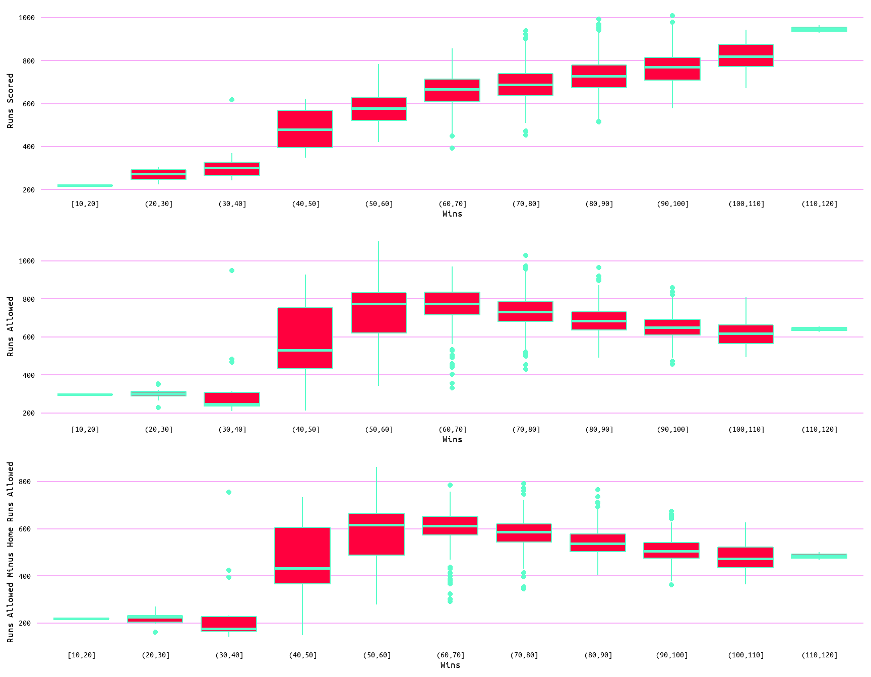
Figure 3: Boxplots for Wins, Runs Scored, Runs Allowed, and Runs Allowed Minus Home Runs Allowed
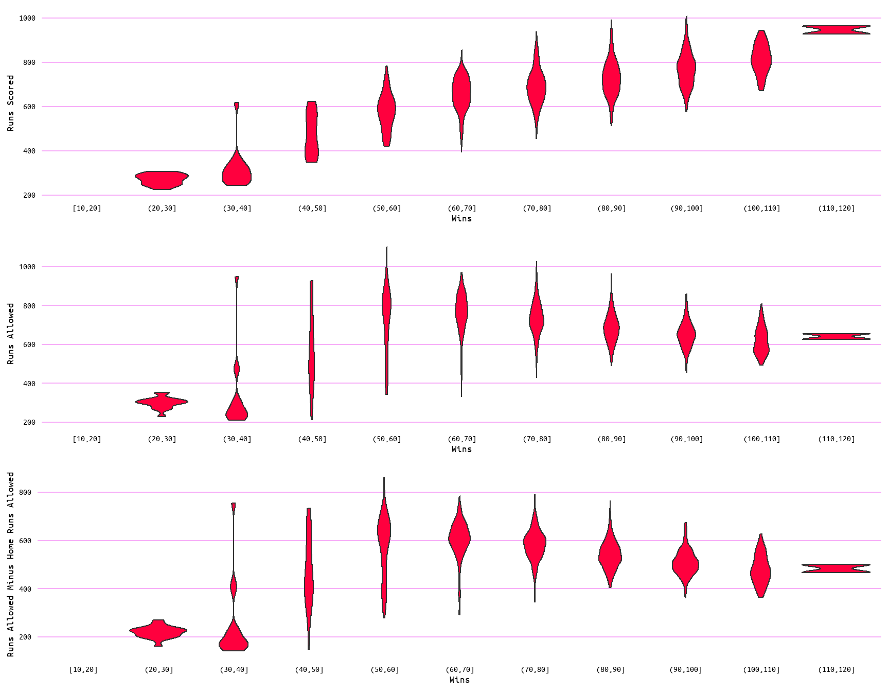
Figure 4: Violin Plots for Wins, Runs Scored, Runs Allowed, and Runs Allowed Minus Home Runs Allowed
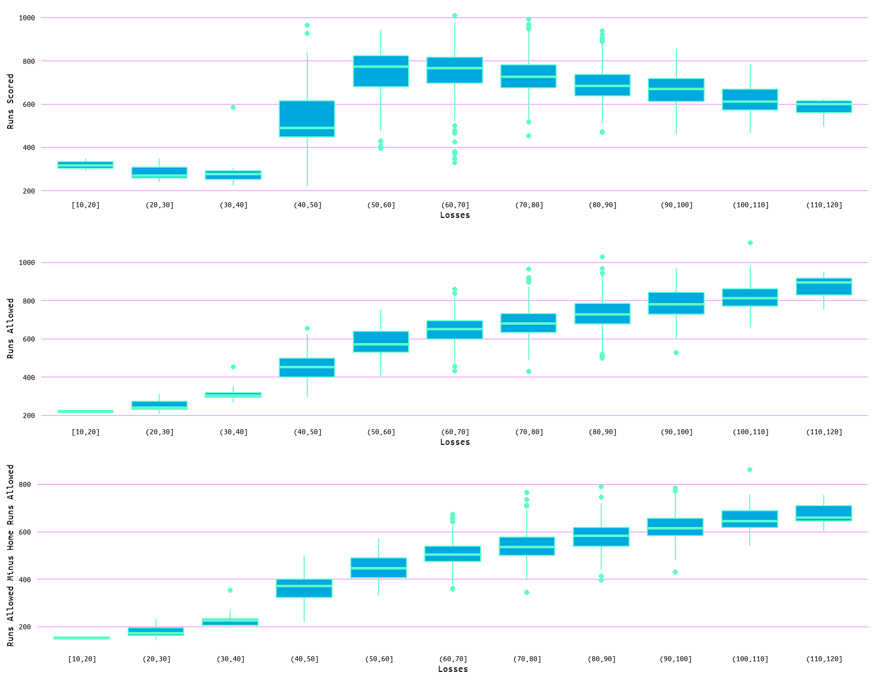
Figure 5: Boxplots for Losses and Runs Scored, Runs Allowed, and Runs Allowed Minus Home Runs Allowed
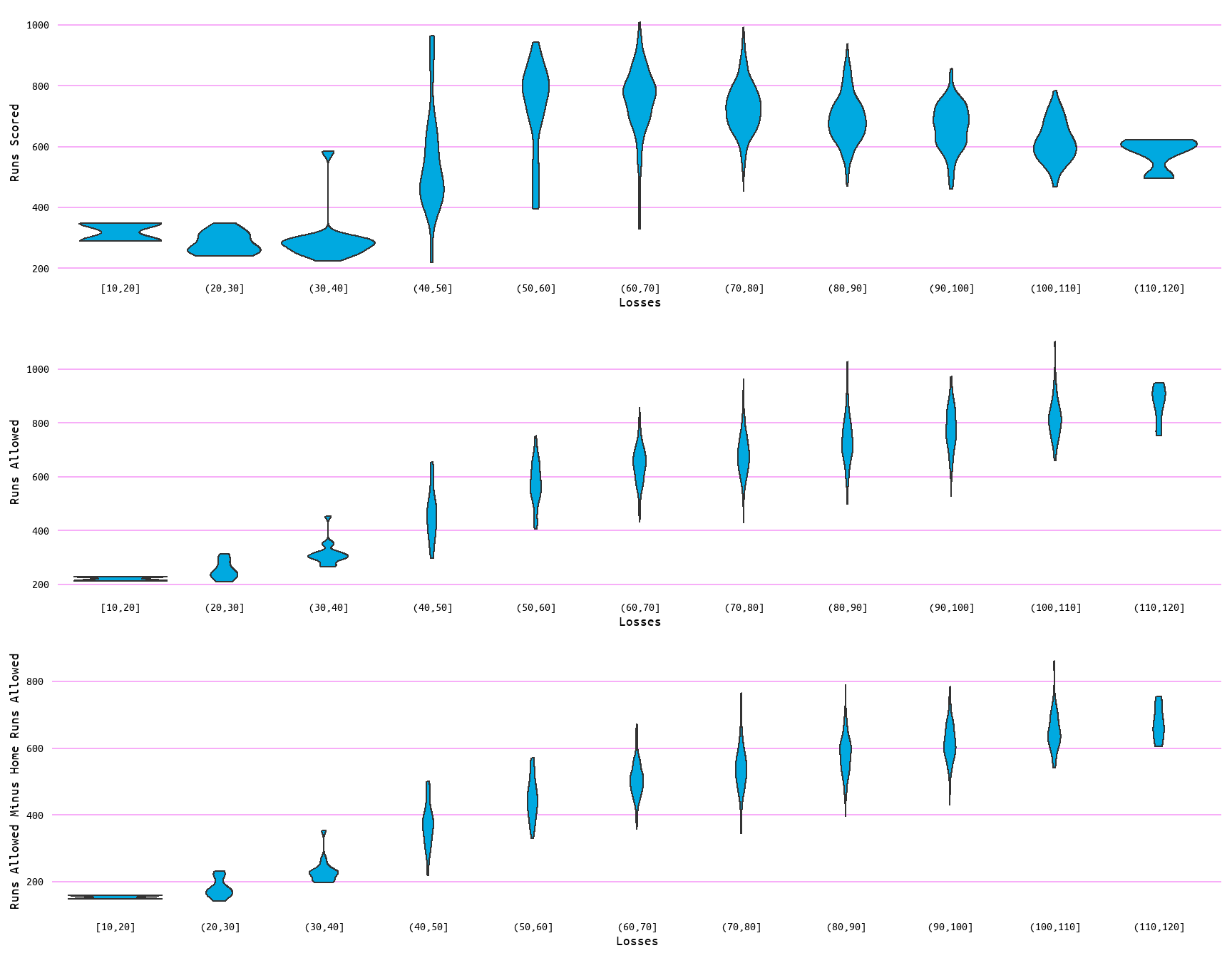
Figure 6: Violin Plots for Losses and Runs Scored, Runs Allowed, and Runs Allowed Minus Home Runs Allowed
Wins Models
Wins ~ Runs Scored
The first regression model used wins as the dependent or outcome variable and runs scored as the independent or predictor variable. As wins is a numerical value, linear regression was used. This model returned a coefficient of determination (hereby referred to as R2) of 0.35 (see Table 3), meaning that runs scored accounted for ~35% of the variance in wins. Additionally, it also returned a residual standard error of 10.03 (see Table 3), meaning that the observed wins deviate from the predicted wins by 10.03 units on average. Figure 7 shows the regression plot for this model with the standard error. It can be seen from that plot that the relationship between wins and runs scored is linear.
| r.squared | adj.r.squared | sigma | statistic | p.value | df | logLik | AIC | BIC | deviance | df.residual | nobs |
|---|---|---|---|---|---|---|---|---|---|---|---|
| 0.48 | 0.48 | 10.18 | 1459.94 | 0 | 1 | -5966.45 | 11938.9 | 11955.03 | 165071.4 | 1594 | 1596 |
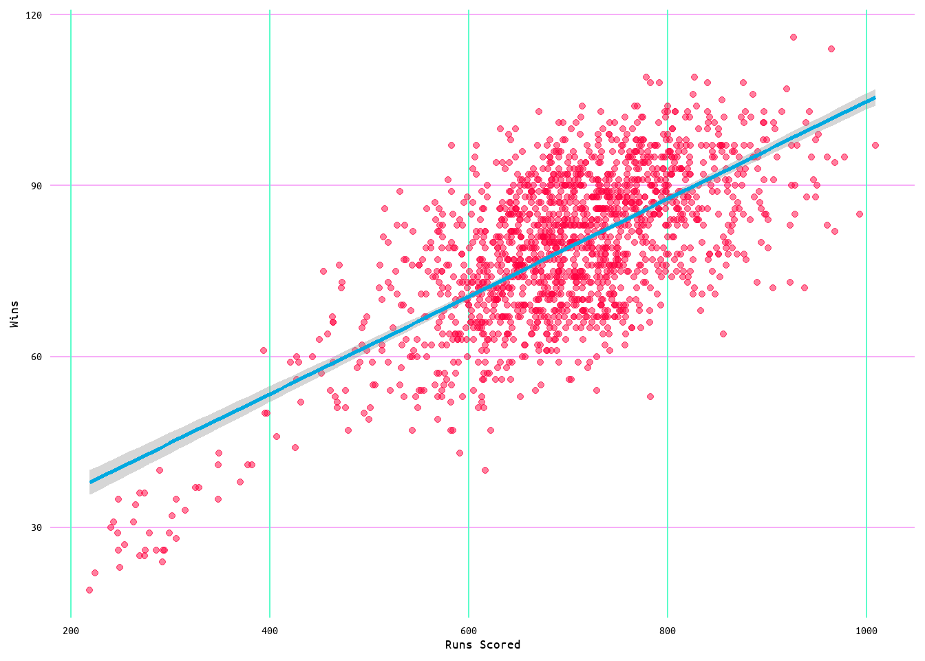
Figure 7: Regression Plot for Wins and Runs Scored Model 1
In further assessing the efficacy of the linear regression model, diagnostic plots were generated to ensure the model met linear regression assumptions. These assumptions being the linearity of the data (the relationship between the dependent and independent variables is assumed to be linear), normality of the residuals (the residual errors are assumed to be distributed normally), the homogeneity of the residuals of variance (the residuals are assumed to have a constant variance), and the independence of residuals error terms (little to no autocorrelation in the residuals). The plots in Figure 8 provided a means of assessing these assumptions.
To assess the assumption of linearity of the data the Residuals vs. Fitted plot in Figure 8 was used. A model that meets this assumption would show a generally flat line. This model met this assumption well, although there appeared to be a slight pattern in the data as the diagnostic line did show a slight curve.
The assumption of normality can be assessed using the Normal Q-Q plot. A model that meets this assumption will have data that falls along the diagnostic line. In the case of this model, this assumption was met.
The assumption of homogeneity can be assessed using the Scale-Location plot, which in the case of this model held fairly well as evidenced by the quite horizontal line.
Additionally, as can be viewed by both the Residuals vs. Fitted plot and the Scale-Location plot, the residuals do show some clustering but overall are fairly well distributed.
Lastly, the Residuals vs. Leverage plot was used to identify cases when extreme values might influence the regression results (outliers). Despite the appearance of outliers as evidenced in Figure 3, no value appeared to exceed three standard deviations, as seen in the Residuals vs. Leverage plot in Figure 8. Suggesting that outliers did not influence the model.
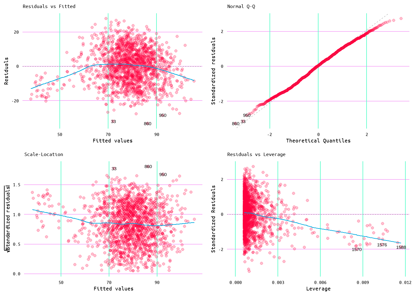
Figure 8: Diagnostic Plots for Wins and Runs Scored Model 1
However, despite the seeming assurance of no influential values, I did also generate another plot to further assess any influential values, given the appearance of outliers in Figure 3. Figure 9 further shows the distribution of residuals as according to Cook’s distance, which reinforces that outliers were not influential for this model.
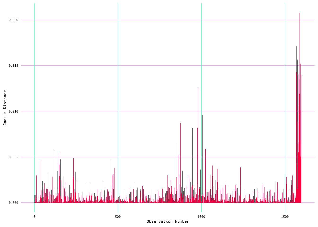
Figure 9: Cook's Distance for Wins Runs Model 1
Although these results suggested that the model performs well, the pattern in the Residuals vs. Fitted plot did present an opportunity to tweak the model for a better performance. To account for this pattern the log of the independent variable (in this case runs) was used. Doing this returned the diagnostic plots seen in Figure 10, which show that the slight curve in Residuals vs. Fitted was corrected, but this also caused the data to be shifted leading to less of a distribution in the residuals (see Figure 10 and Figure 11). Additionally, this marginally improved the model performance by increasing the R2 to 0.36 and producing a residual standard error of 9.97 (see Table 4). However, this improvement may be due to the shift in the distribution of the data as opposed to any improvement in the model. As such, the original model without the use of a log transformed predictor is probably the better of the two models to use.
| r.squared | adj.r.squared | sigma | statistic | p.value | df | logLik | AIC | BIC | deviance | df.residual | nobs |
|---|---|---|---|---|---|---|---|---|---|---|---|
| 0.51 | 0.51 | 9.91 | 1629.41 | 0 | 1 | -5923.35 | 11852.7 | 11868.83 | 156392.5 | 1594 | 1596 |
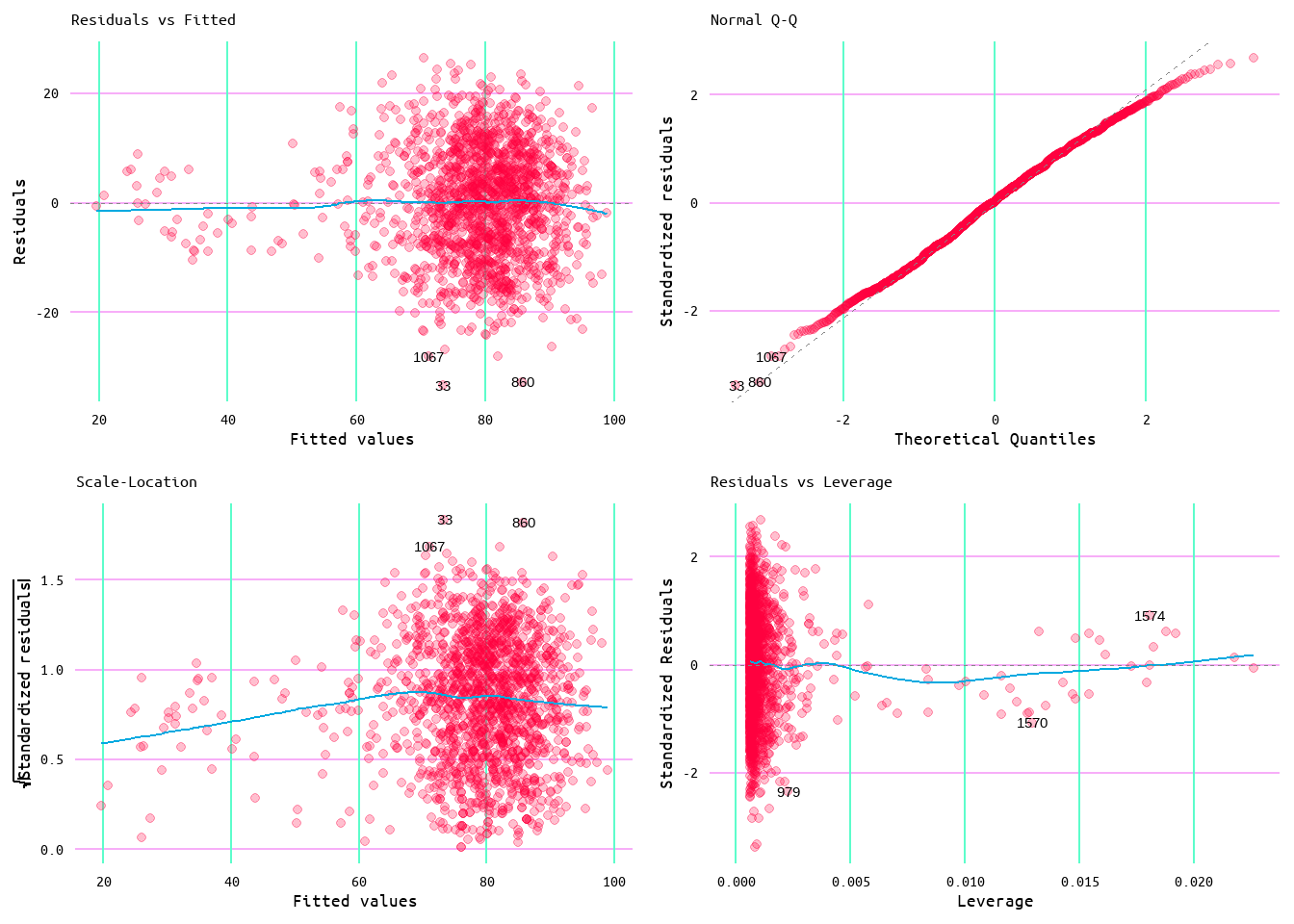
Figure 10: Diagnostic Plots for Wins and Runs Scored Model 2
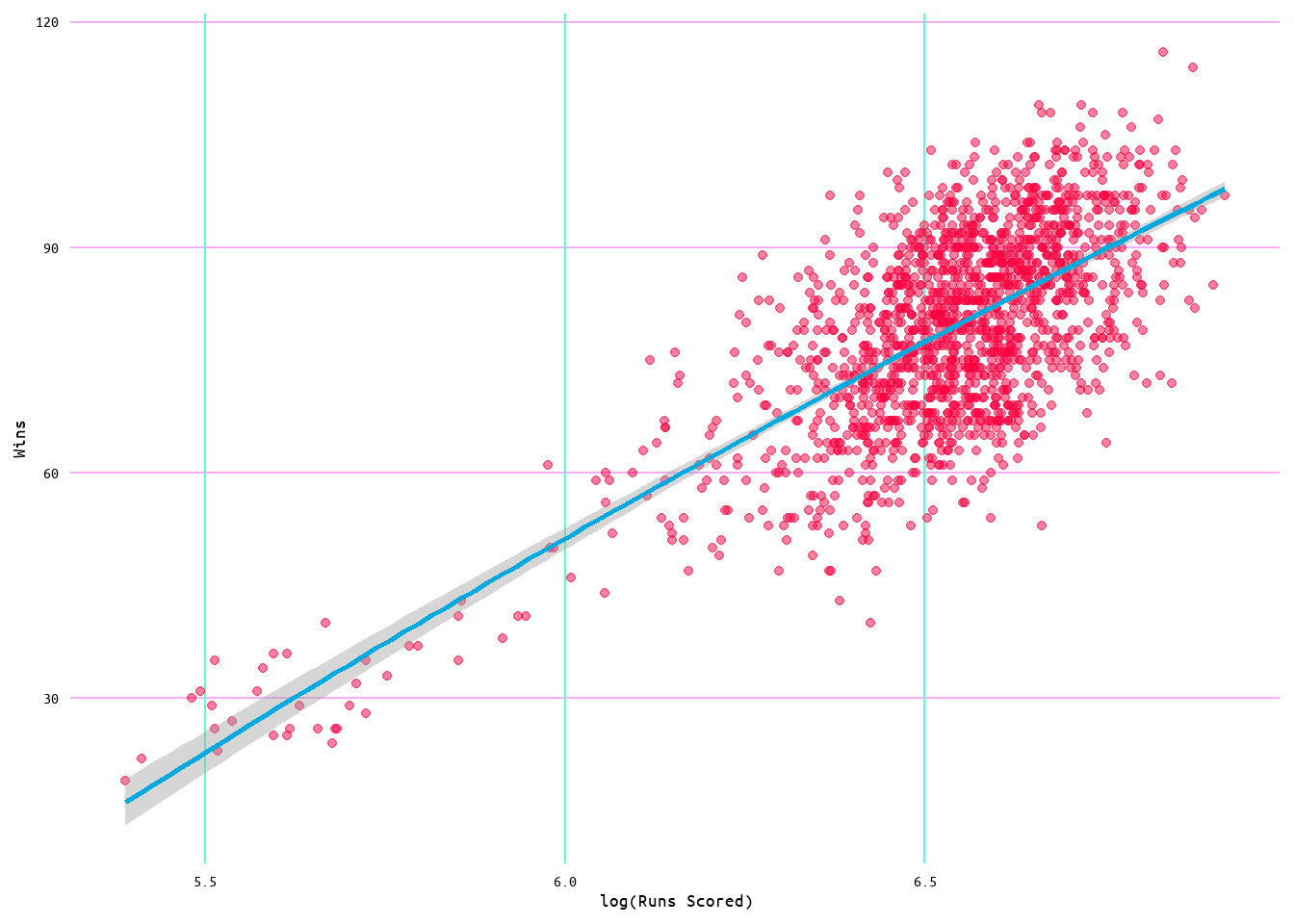
Figure 11: Regression Plot for Wins and Runs Scored Model 2
Wins ~ Runs Allowed Model
As the purpose of this was to also explore wins and runs allowed, a model was also generated using runs allowed as a predictor of wins. The initial model returned an R2 value of 0.1 (meaning that runs allowed accounts for ~10% of variance in wins) with a residual standard error of 11.83 (see Table 5). Looking at Figure 12, the relationship between wins and runs allowed appears to be linear; however, looking at the diagnostic plots in Figure 13, it can be seen that the model does not quite meet every linear regression assumption. Moreover, looking at Figure 14 it looks as if there are some influential values that may be affecting the model.
| r.squared | adj.r.squared | sigma | statistic | p.value | df | logLik | AIC | BIC | deviance | df.residual | nobs |
|---|---|---|---|---|---|---|---|---|---|---|---|
| 0 | 0 | 14.09 | 0.03 | 0.87 | 1 | -6485.29 | 12976.57 | 12992.7 | 316254.5 | 1594 | 1596 |
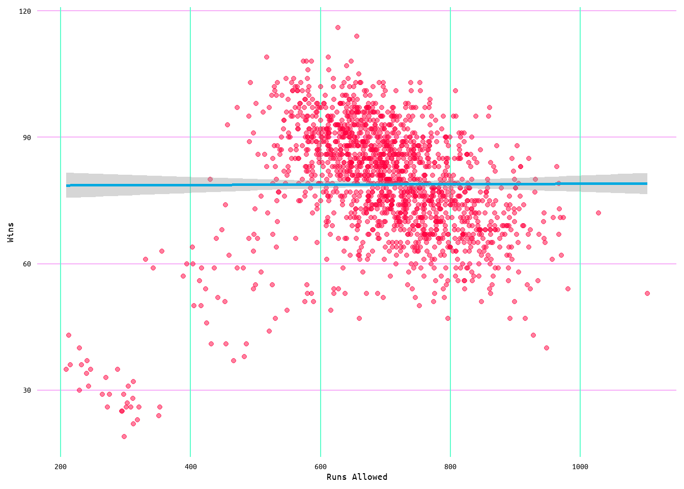
Figure 12: Regression Plot for Wins and Runs Allowed Model 1
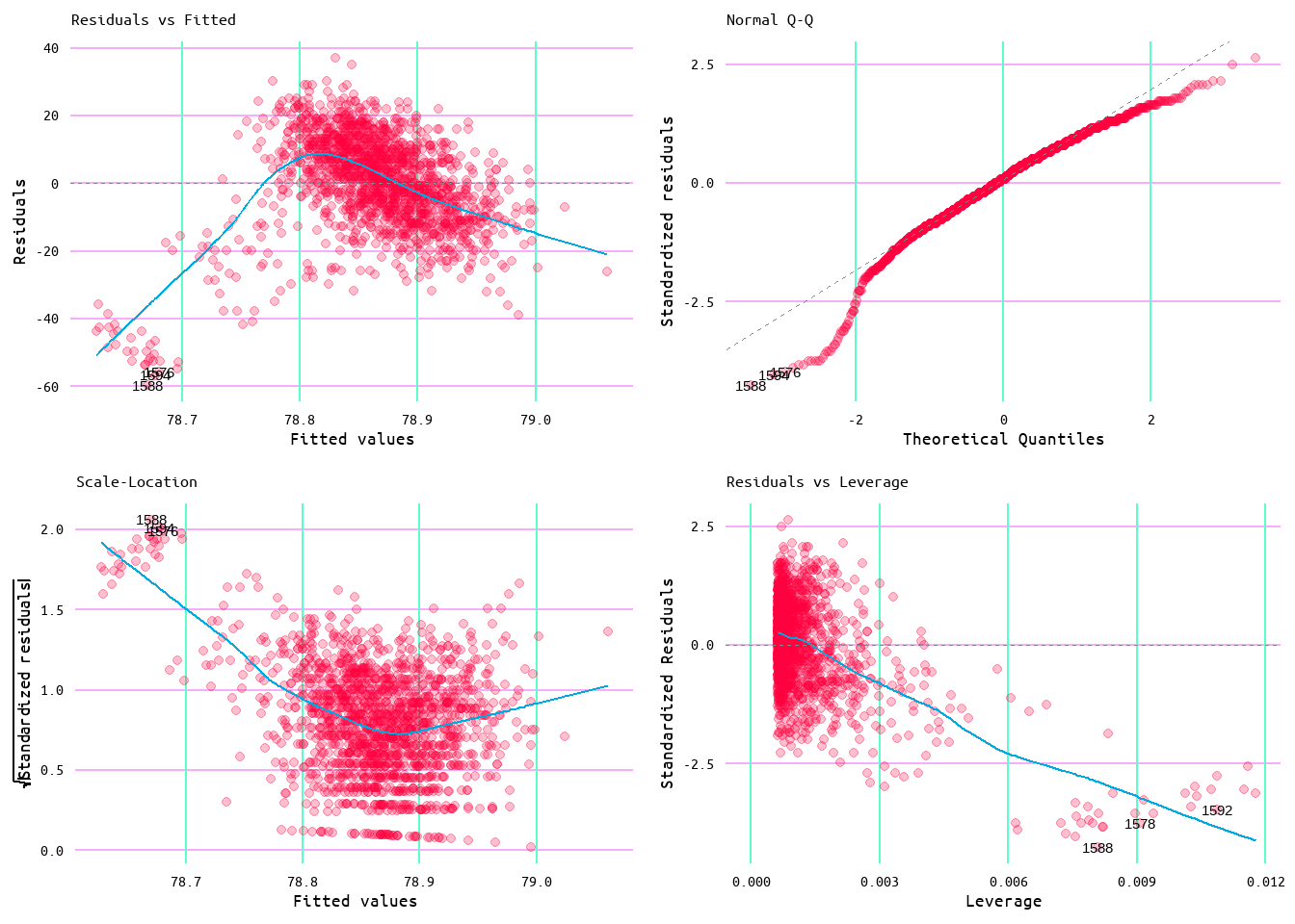
Figure 13: Diagnostic Plots for Wins and Runs Allowed Model 1
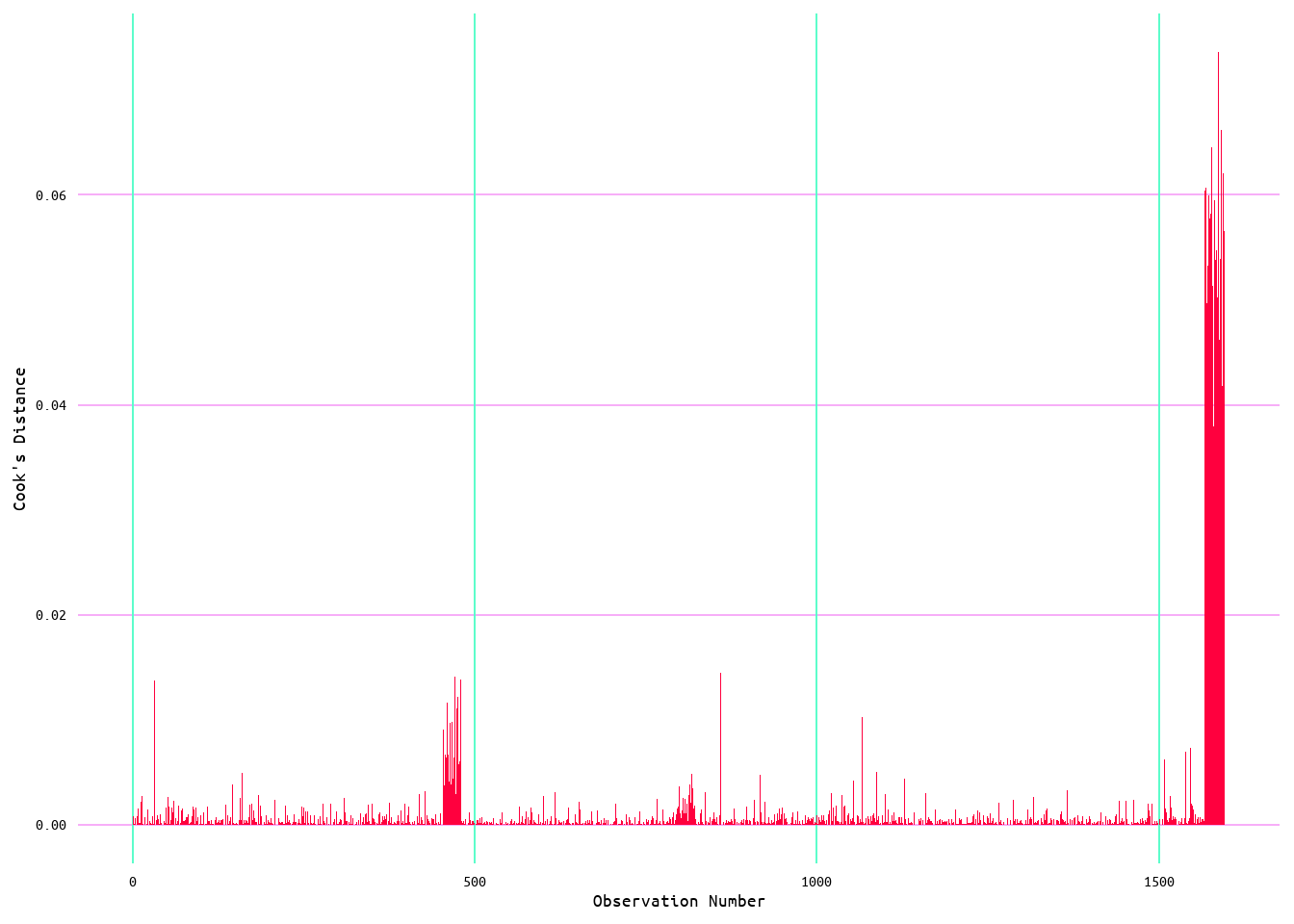
Figure 14: Cook's Distance for Wins and Runs Allowed Model 1
Because of the influential values, I decided to cap the outliers for runs allowed such that those observations outside the lower limit were capped with the 5th percentile value, and those that fall outside the upper limit were capped with the 95th percentile value. A summary table of the dataset with capped outliers is displayed in Table 6, while a comparison of the original values is displayed in Table 7. With capped values, runs allowed now has a minimum of 453 runs as compared to 331 runs and a max of 958 runs as compared to 1103 runs; however, the median remained the same at 702 runs while the mean decreased by 1 from 706 runs to 705 runs. Additionally, it can be seen in Figure 15 that the distribution of the capped runs allowed is still quite Gaussian as compared to the original distribution.
| W | L | R | RA | RA_MHRA | |
|---|---|---|---|---|---|
| Min. : 19.00 | Min. : 17.00 | Min. : 219.0 | Min. :442.0 | Min. :141.0 | |
| 1st Qu.: 71.00 | 1st Qu.: 71.00 | 1st Qu.: 640.0 | 1st Qu.:638.0 | 1st Qu.:503.0 | |
| Median : 80.00 | Median : 79.00 | Median : 703.0 | Median :700.0 | Median :556.0 | |
| Mean : 78.86 | Mean : 78.86 | Mean : 697.1 | Mean :702.2 | Mean :550.3 | |
| 3rd Qu.: 89.00 | 3rd Qu.: 88.00 | 3rd Qu.: 767.2 | 3rd Qu.:769.0 | 3rd Qu.:608.0 | |
| Max. :116.00 | Max. :120.00 | Max. :1009.0 | Max. :964.0 | Max. :862.0 |
| W | L | R | RA | RA_MHRA | |
|---|---|---|---|---|---|
| Min. : 19.00 | Min. : 17.00 | Min. : 219.0 | Min. : 209.0 | Min. :141.0 | |
| 1st Qu.: 71.00 | 1st Qu.: 71.00 | 1st Qu.: 640.0 | 1st Qu.: 638.0 | 1st Qu.:503.0 | |
| Median : 80.00 | Median : 79.00 | Median : 703.0 | Median : 700.0 | Median :556.0 | |
| Mean : 78.86 | Mean : 78.86 | Mean : 697.1 | Mean : 697.1 | Mean :550.3 | |
| 3rd Qu.: 89.00 | 3rd Qu.: 88.00 | 3rd Qu.: 767.2 | 3rd Qu.: 769.0 | 3rd Qu.:608.0 | |
| Max. :116.00 | Max. :120.00 | Max. :1009.0 | Max. :1103.0 | Max. :862.0 |
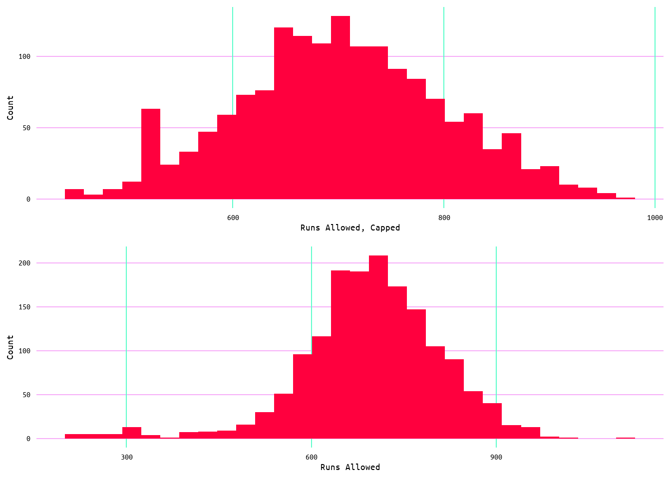
Figure 15: Distribution Comparison of Capped Runs Allowed Values and Unadjusted Runs Allowed Values
I also generated a model using the capped dataset to see if this improved the model results at all. This model returned an R2 of 0.12, a slight improvement over the original R2 of 0.1, and a residual standard error of 11.65, which is fairly close to the original value of 11.83 (see Table 8). Additionally, as seen in Figure 16, the model meets the linear regression assumptions much better than it had before. Additionally, there appears to be a good distribution of the residuals. However, looking at Figure 17, there still appears to be some issue with outliers and in Figure 18 there is an obvious pattern created by the capped values. Effectively, runs allowed is not enough by itself to account for wins.
| r.squared | adj.r.squared | sigma | statistic | p.value | df | logLik | AIC | BIC | deviance | df.residual | nobs |
|---|---|---|---|---|---|---|---|---|---|---|---|
| 0.03 | 0.03 | 13.89 | 44.93 | 0 | 1 | -6463.12 | 12932.24 | 12948.36 | 307590.3 | 1594 | 1596 |
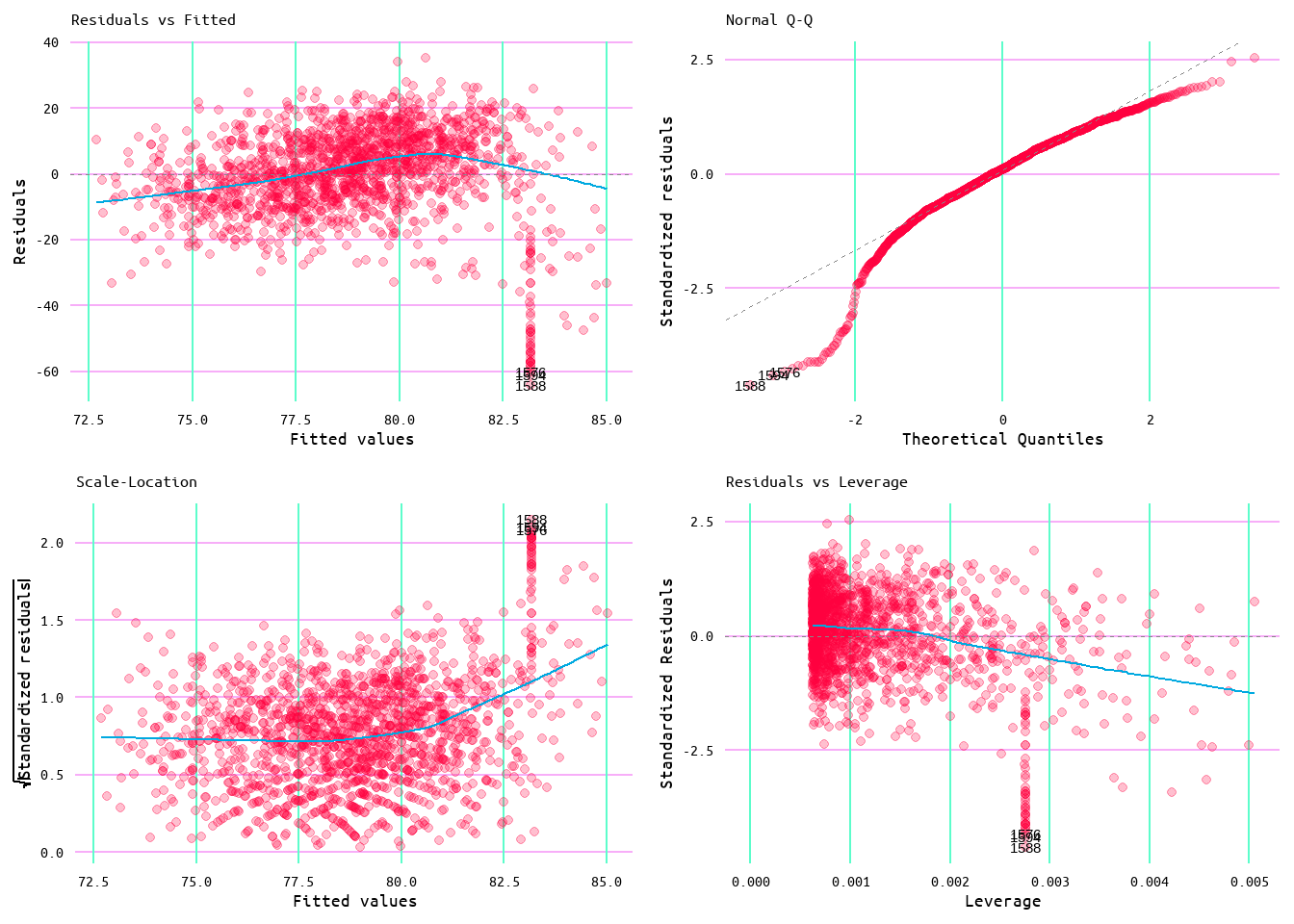
Figure 16: Diagnostic Plots for Wins and Runs Allowed Model 2
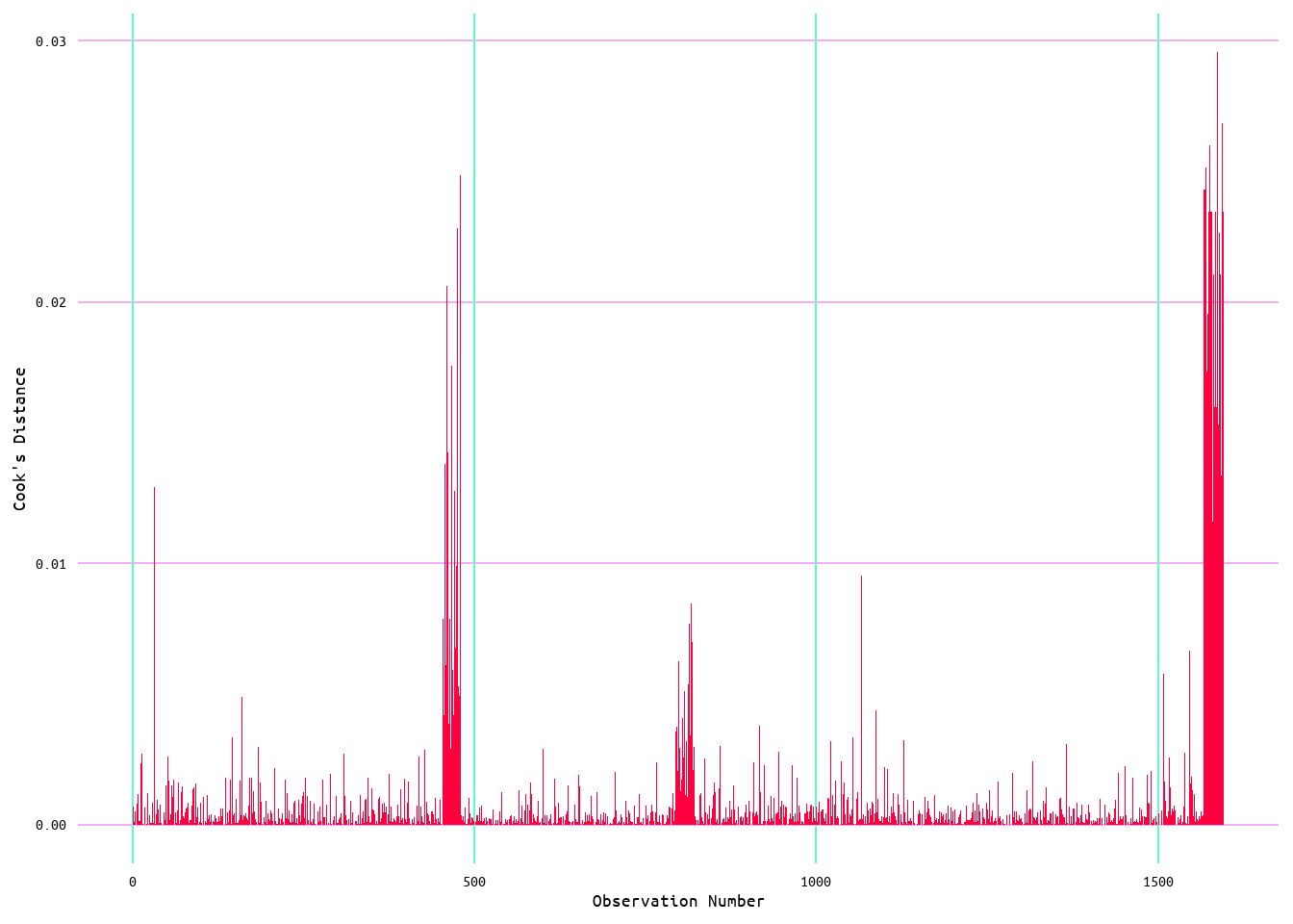
Figure 17: Cook's Distance for Wins Runs Allowed Model 2
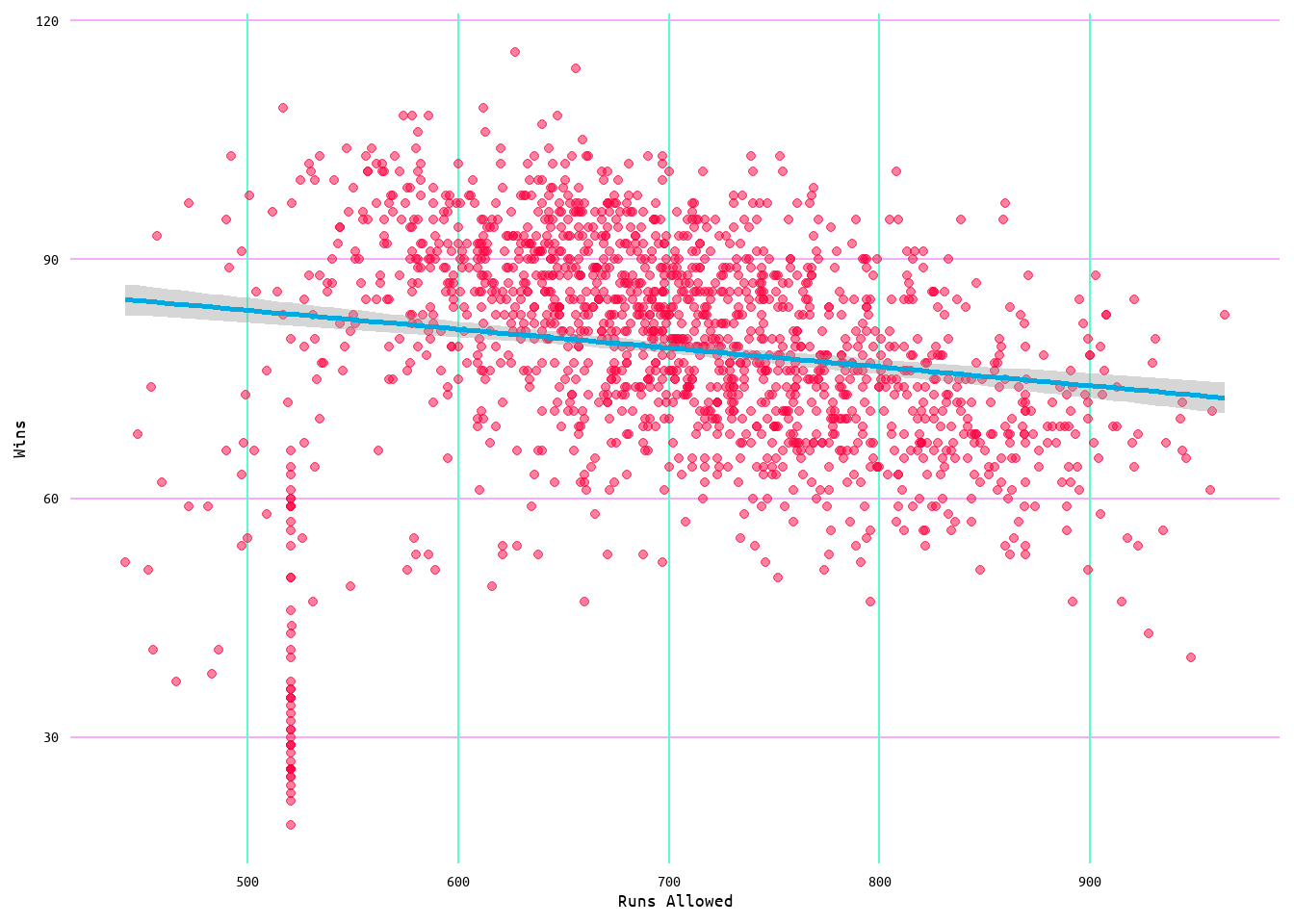
Figure 18: Regression Plot for Wins and Runs Allowed Model 2
Wins ~ Runs Allowed Minus Home Runs Allowed Model
Lastly, because pitching is so involved with runs allowed I removed home runs allowed to somewhat (although weakly) accommodate for this. An initial model returned an R2 of 0.13 with a residual standard error of 11.58 (see Table 9). Meaning that runs allowed minus home runs allowed accounts for ~13% of the variance in wins. An improvement over the runs allowed model.
Looking at Figure 19, there does appear to be a fairly linear relationship between runs allowed minus home runs allowed and wins. However, looking at the diagnostic plots in Figure 20, there appears to be the same issues with this model as there were with the runs allowed model. Which makes sense. Looking at Figure 21, this again appears to be an issue with influential values.
| r.squared | adj.r.squared | sigma | statistic | p.value | df | logLik | AIC | BIC | deviance | df.residual | nobs |
|---|---|---|---|---|---|---|---|---|---|---|---|
| 0 | 0 | 14.08 | 0.51 | 0.48 | 1 | -6485.04 | 12976.09 | 12992.21 | 316158.5 | 1594 | 1596 |
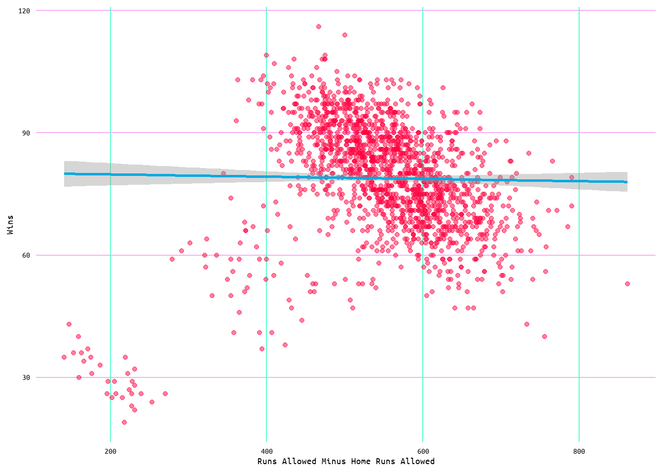
Figure 19: Regression Plot for Wins and Runs Allowed Minus Home Runs Allowed Model 1
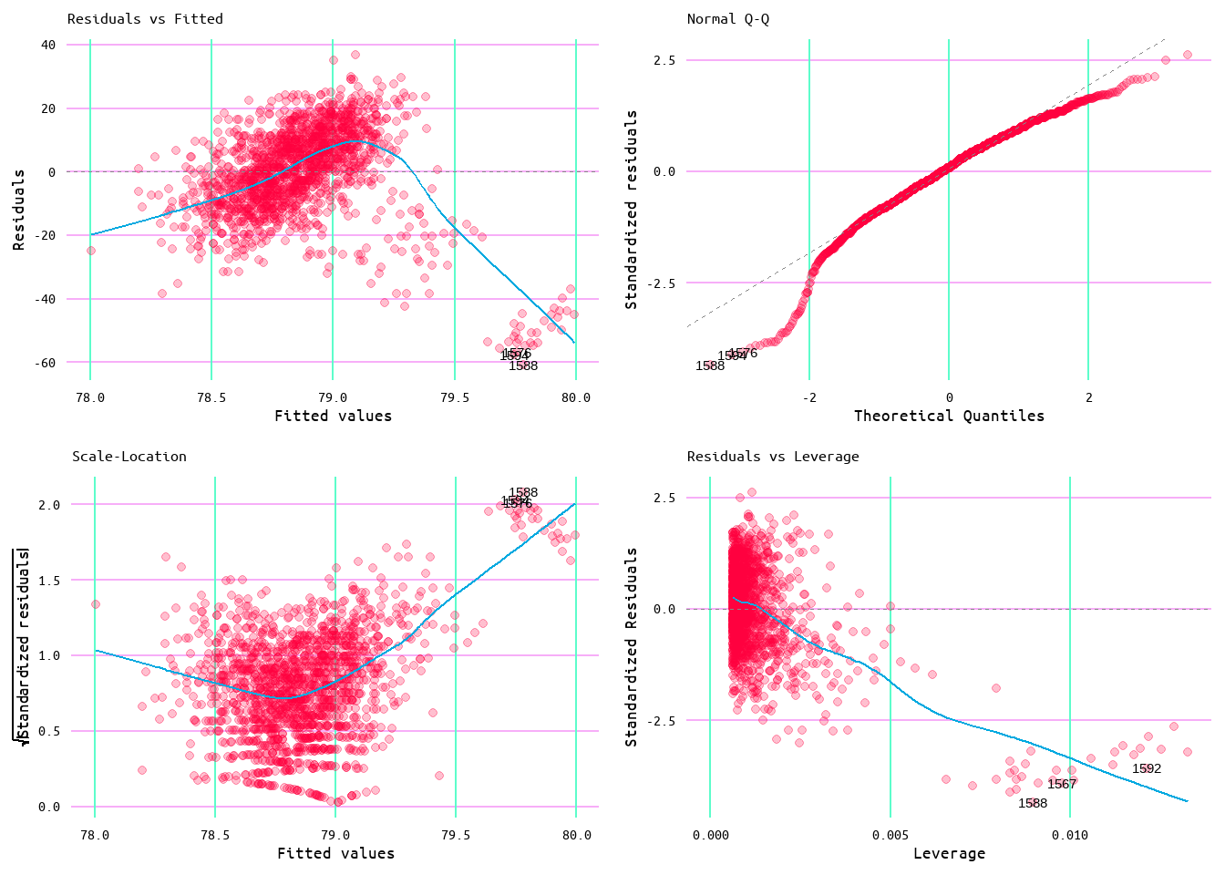
Figure 20: Diagnostic Plots for Wins and Runs Allowed Minus Home Runs Allowed Model 1
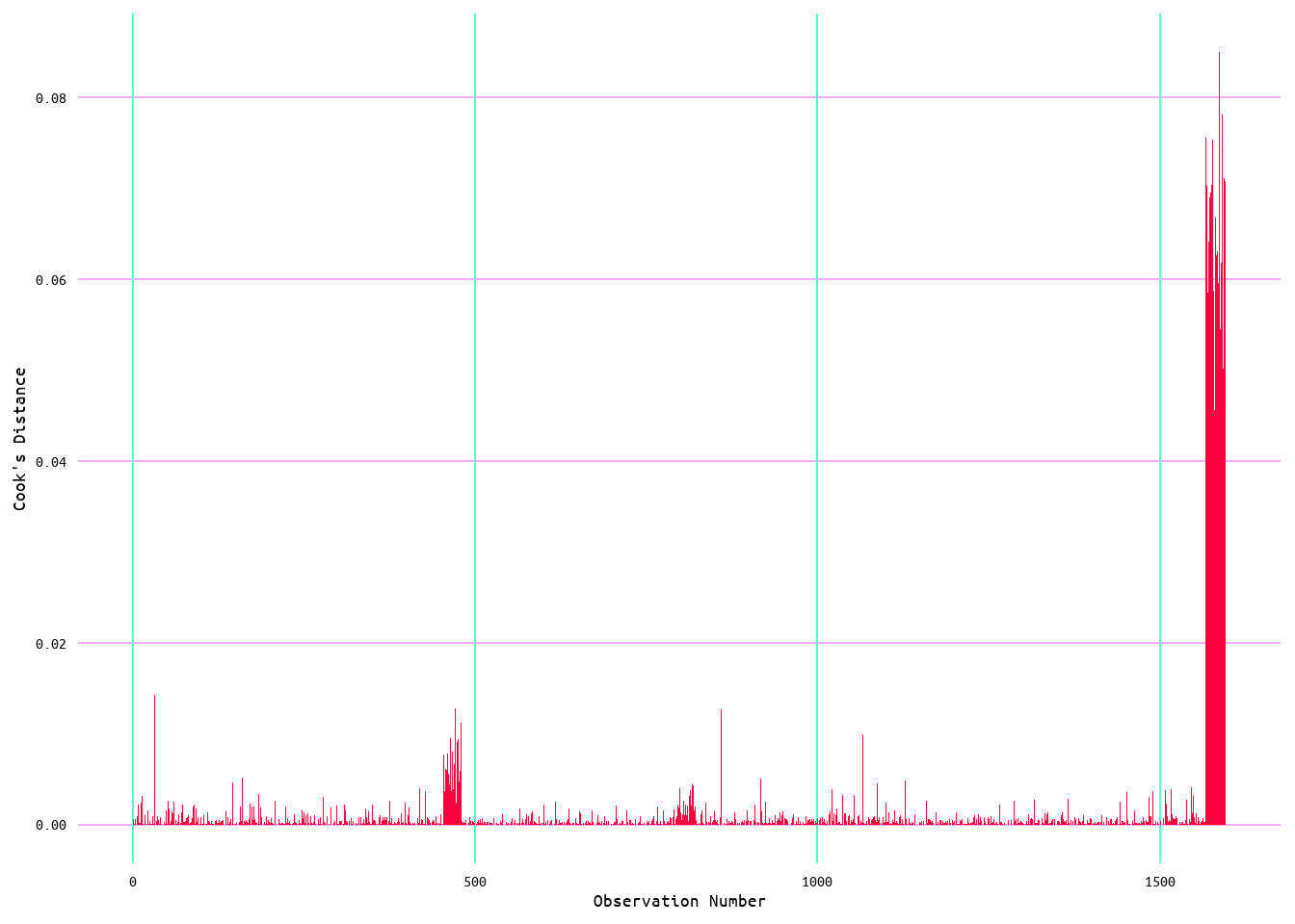
Figure 21: Cook's Distance for Wins Runs Allowed Minus Home Runs Allowed Model 1
As such, the values for runs allowed minus home runs allowed were capped using the same methods as with runs allowed. Table 10 shows the capped values for runs allowed minus home runs allowed, while Table 11 shows the original values. Looking at these tables it can be seen that the minimum value for runs allowed minus home runs allowed increased from 279 runs to 354 runs, while the max value decreased from 862 runs to 761 runs. Moreover, the median and mean stayed the same at 557 runs, while the distribution for runs allowed minus home runs allowed stayed Gaussian (Figure 22).
| W | L | R | RA | RA_MHRA | |
|---|---|---|---|---|---|
| Min. : 19.00 | Min. : 17.00 | Min. : 219.0 | Min. :442.0 | Min. :350.0 | |
| 1st Qu.: 71.00 | 1st Qu.: 71.00 | 1st Qu.: 640.0 | 1st Qu.:638.0 | 1st Qu.:503.0 | |
| Median : 80.00 | Median : 79.00 | Median : 703.0 | Median :700.0 | Median :556.0 | |
| Mean : 78.86 | Mean : 78.86 | Mean : 697.1 | Mean :702.2 | Mean :554.3 | |
| 3rd Qu.: 89.00 | 3rd Qu.: 88.00 | 3rd Qu.: 767.2 | 3rd Qu.:769.0 | 3rd Qu.:608.0 | |
| Max. :116.00 | Max. :120.00 | Max. :1009.0 | Max. :964.0 | Max. :761.0 |
| W | L | R | RA | RA_MHRA | |
|---|---|---|---|---|---|
| Min. : 19.00 | Min. : 17.00 | Min. : 219.0 | Min. : 209.0 | Min. :141.0 | |
| 1st Qu.: 71.00 | 1st Qu.: 71.00 | 1st Qu.: 640.0 | 1st Qu.: 638.0 | 1st Qu.:503.0 | |
| Median : 80.00 | Median : 79.00 | Median : 703.0 | Median : 700.0 | Median :556.0 | |
| Mean : 78.86 | Mean : 78.86 | Mean : 697.1 | Mean : 697.1 | Mean :550.3 | |
| 3rd Qu.: 89.00 | 3rd Qu.: 88.00 | 3rd Qu.: 767.2 | 3rd Qu.: 769.0 | 3rd Qu.:608.0 | |
| Max. :116.00 | Max. :120.00 | Max. :1009.0 | Max. :1103.0 | Max. :862.0 |
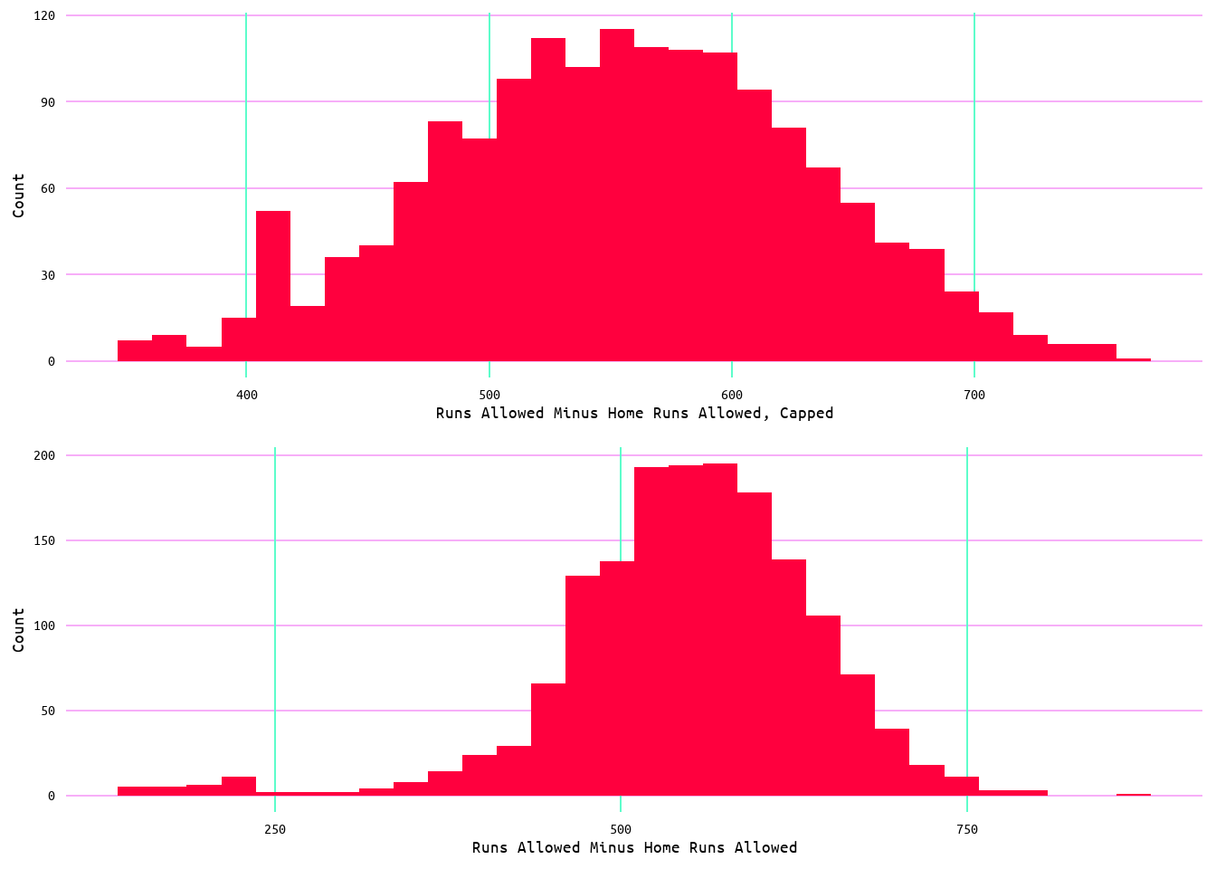
Figure 22: Distribution Comparison of Capped and Unadjusted Runs Allowed Minus Home Runs Allowed
The model using the capped values, returned an R2 value of 0.15, an improvement over the original model, and a residual standard error of 11.46, which was still fairly similar to the original of 11.58 (see Table 12). Moreover, looking at the diagnostic plots in Figure 23, improvements can be seen in terms of the assumptions, but there still appears to be some issues that also appeared in the runs allowed model (see Figure 24 and Figure 25). Which again makes sense given the construction of this variable.
| r.squared | adj.r.squared | sigma | statistic | p.value | df | logLik | AIC | BIC | deviance | df.residual | nobs |
|---|---|---|---|---|---|---|---|---|---|---|---|
| 0.04 | 0.04 | 13.81 | 65.08 | 0 | 1 | -6453.36 | 12912.72 | 12928.85 | 303852.8 | 1594 | 1596 |
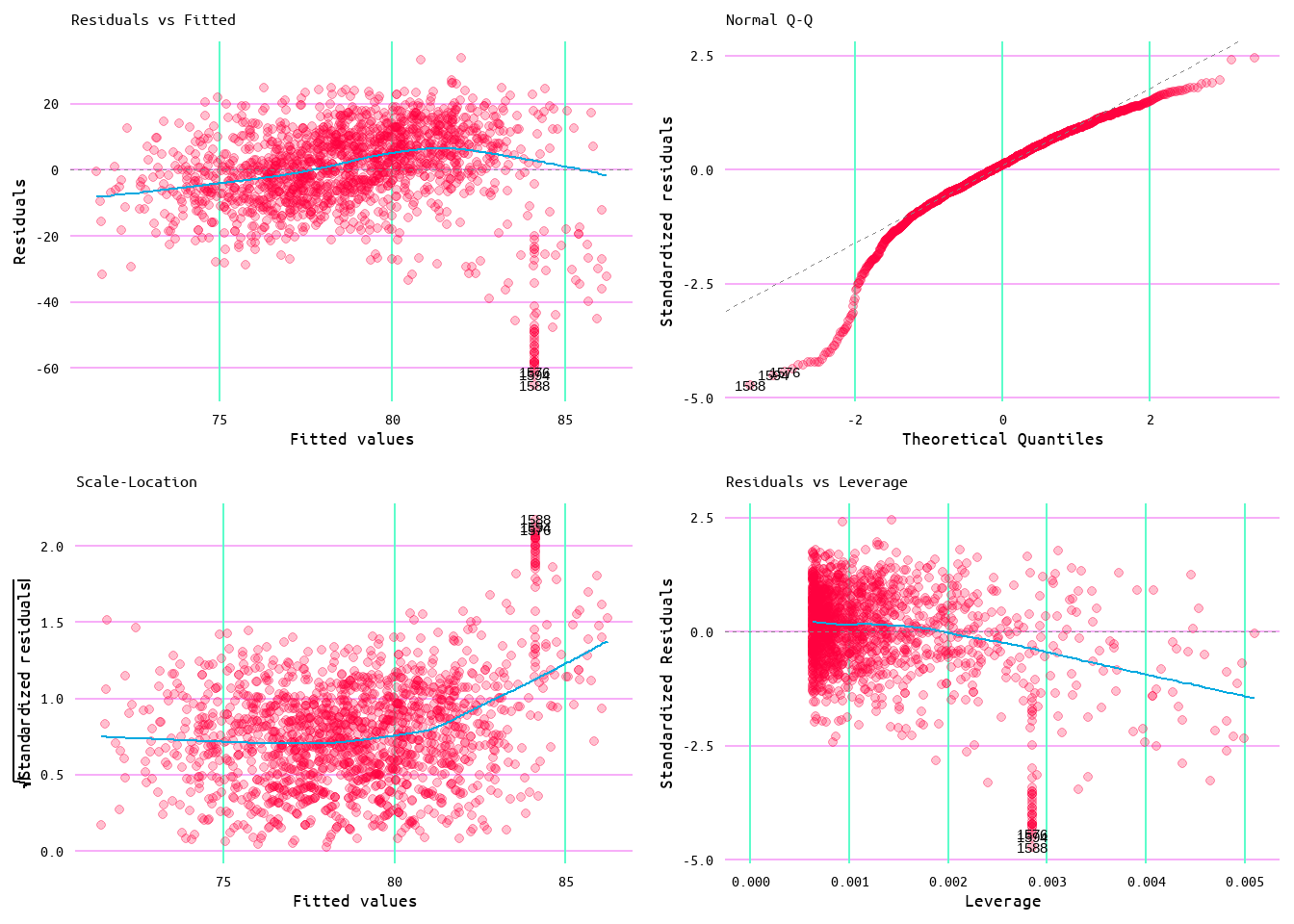
Figure 23: Diagnostic Plots for Wins and Runs Allowed Minus Home Runs Allowed Model 2
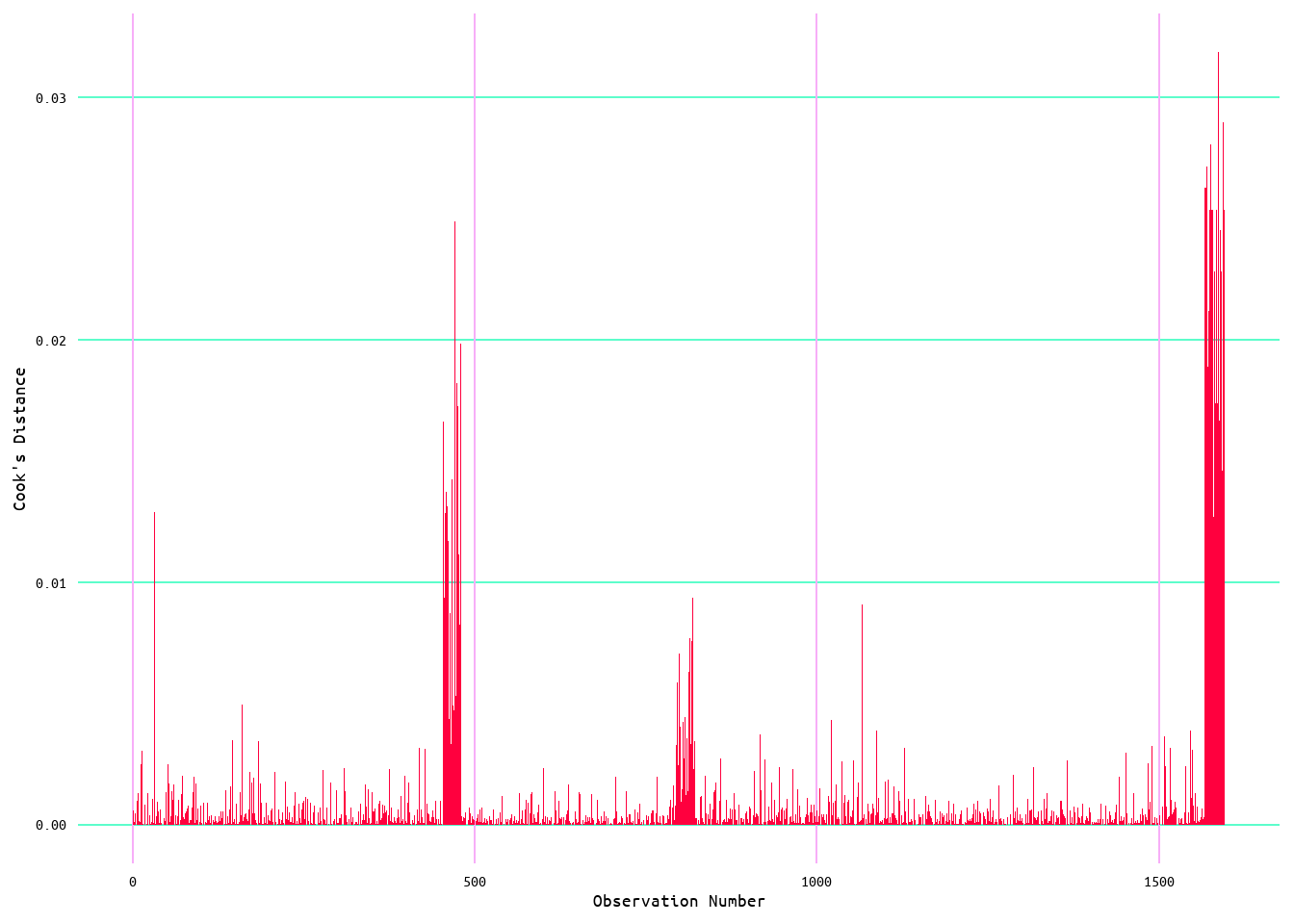
Figure 24: Cook's Distance for Wins Runs Allowed Model 2
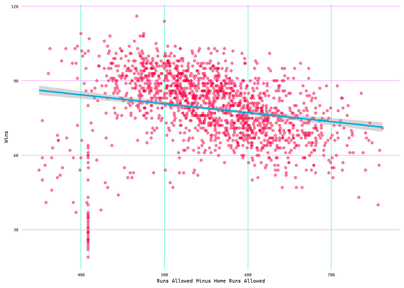
Figure 25: Regression Plot for Wins and Runs Allowed Minus Home Runs Allowed Model 2
Losses Models
Losses ~ Runs Scored Model
Moving onto losses. Using runs scored as the independent variable initially produces an R2 value of 0.07, meaning that runs scored account for ~7% of the variance in losses, with a residual standard error of 11.94 (see Table 13). However, looking at the diagnostic plots in Figure 27, it can be seen that similar issues as found in the wins and runs allowed models appear in this model as well. Indeed, looking at Figure 26, the distribution of points in the relationship between losses and runs scored is very similar to that seen in Figure 12 with wins and runs allowed. Furthermore, looking at Figure 27 and Figure 28, the issue once again appears to be one of influential values.
As such, the same capping process used for both runs allowed and runs allowed minus home runs allowed was used. This adjusted the minimum value of runs from 329 runs to 458 runs, and the maximum value of runs from 1009 runs to 952 runs (see Table 14 and Table 15). As well, in the adjustment the median remained the same at 706 runs while the mean value of runs increased from 705 to 706 (Table 14 and Table 15). Additionally, the distribution of the values remained Gaussian after having capped the outlier values for runs scored (Figure 29).
Running the losses and runs scored model again, but now with the capped values, returned an R2 of ~0.1 (rounded up from 0.0951969) with a residual standard error of 11.79 (see Table 16). Which puts the model around the same as the original wins and runs allowed model in terms of accounting for variance. Looking at Figure 30, the diagnostic plots for this model show that the assumptions are more closely met than the original losses and runs scored model. Additionally, the results closely resemble those seen with the wins and runs allowed model. Moreover, the same pattern that appeared in the regression plot for wins and runs allowed similarly appears in the regression plot for losses, runs scored after capping the values (see Figure 31). While the results of capping influential outliers does show an improvement in the model regarding inference, it should be noted that the results of the original model suggest that it would be better served by incorporating more variables rather than attempting to continue with runs scored alone.
| r.squared | adj.r.squared | sigma | statistic | p.value | df | logLik | AIC | BIC | deviance | df.residual | nobs |
|---|---|---|---|---|---|---|---|---|---|---|---|
| 0 | 0 | 14.03 | 2.93 | 0.09 | 1 | -6478.93 | 12963.85 | 12979.98 | 313744.5 | 1594 | 1596 |
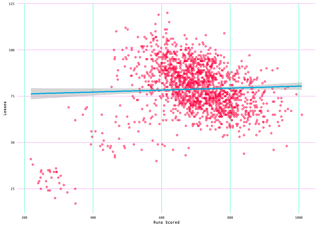
Figure 26: Regression Plot for Losses and Runs Scored Model 1
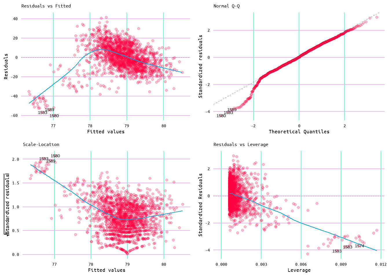
Figure 27: Diagnostic Plots for Wins and Runs Allowed Model 4
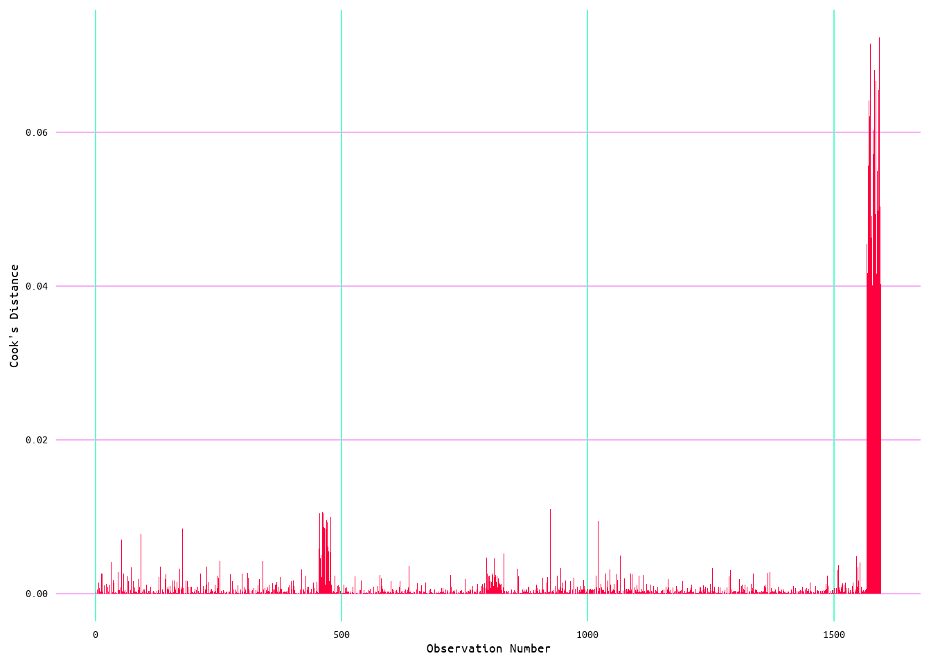
Figure 28: Cook's Distance for Wins Runs Allowed Model 1
| W | L | R | RA | RA_MHRA | |
|---|---|---|---|---|---|
| Min. : 19.00 | Min. : 17.00 | Min. :450.0 | Min. :442.0 | Min. :350.0 | |
| 1st Qu.: 71.00 | 1st Qu.: 71.00 | 1st Qu.:640.0 | 1st Qu.:638.0 | 1st Qu.:503.0 | |
| Median : 80.00 | Median : 79.00 | Median :703.0 | Median :700.0 | Median :556.0 | |
| Mean : 78.86 | Mean : 78.86 | Mean :702.0 | Mean :702.2 | Mean :554.3 | |
| 3rd Qu.: 89.00 | 3rd Qu.: 88.00 | 3rd Qu.:767.2 | 3rd Qu.:769.0 | 3rd Qu.:608.0 | |
| Max. :116.00 | Max. :120.00 | Max. :952.0 | Max. :964.0 | Max. :761.0 |
| W | L | R | RA | RA_MHRA | |
|---|---|---|---|---|---|
| Min. : 19.00 | Min. : 17.00 | Min. : 219.0 | Min. : 209.0 | Min. :141.0 | |
| 1st Qu.: 71.00 | 1st Qu.: 71.00 | 1st Qu.: 640.0 | 1st Qu.: 638.0 | 1st Qu.:503.0 | |
| Median : 80.00 | Median : 79.00 | Median : 703.0 | Median : 700.0 | Median :556.0 | |
| Mean : 78.86 | Mean : 78.86 | Mean : 697.1 | Mean : 697.1 | Mean :550.3 | |
| 3rd Qu.: 89.00 | 3rd Qu.: 88.00 | 3rd Qu.: 767.2 | 3rd Qu.: 769.0 | 3rd Qu.:608.0 | |
| Max. :116.00 | Max. :120.00 | Max. :1009.0 | Max. :1103.0 | Max. :862.0 |
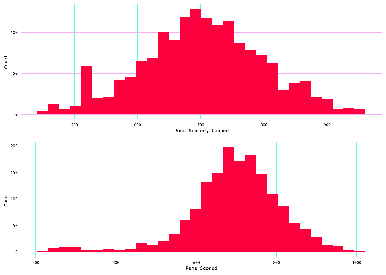
Figure 29: Distribtion Comparison of Capped and Unadjusted Runs Scored Values
| r.squared | adj.r.squared | sigma | statistic | p.value | df | logLik | AIC | BIC | deviance | df.residual | nobs |
|---|---|---|---|---|---|---|---|---|---|---|---|
| 0.01 | 0.01 | 13.94 | 23.1 | 0 | 1 | -6468.91 | 12943.82 | 12959.94 | 309830.7 | 1594 | 1596 |
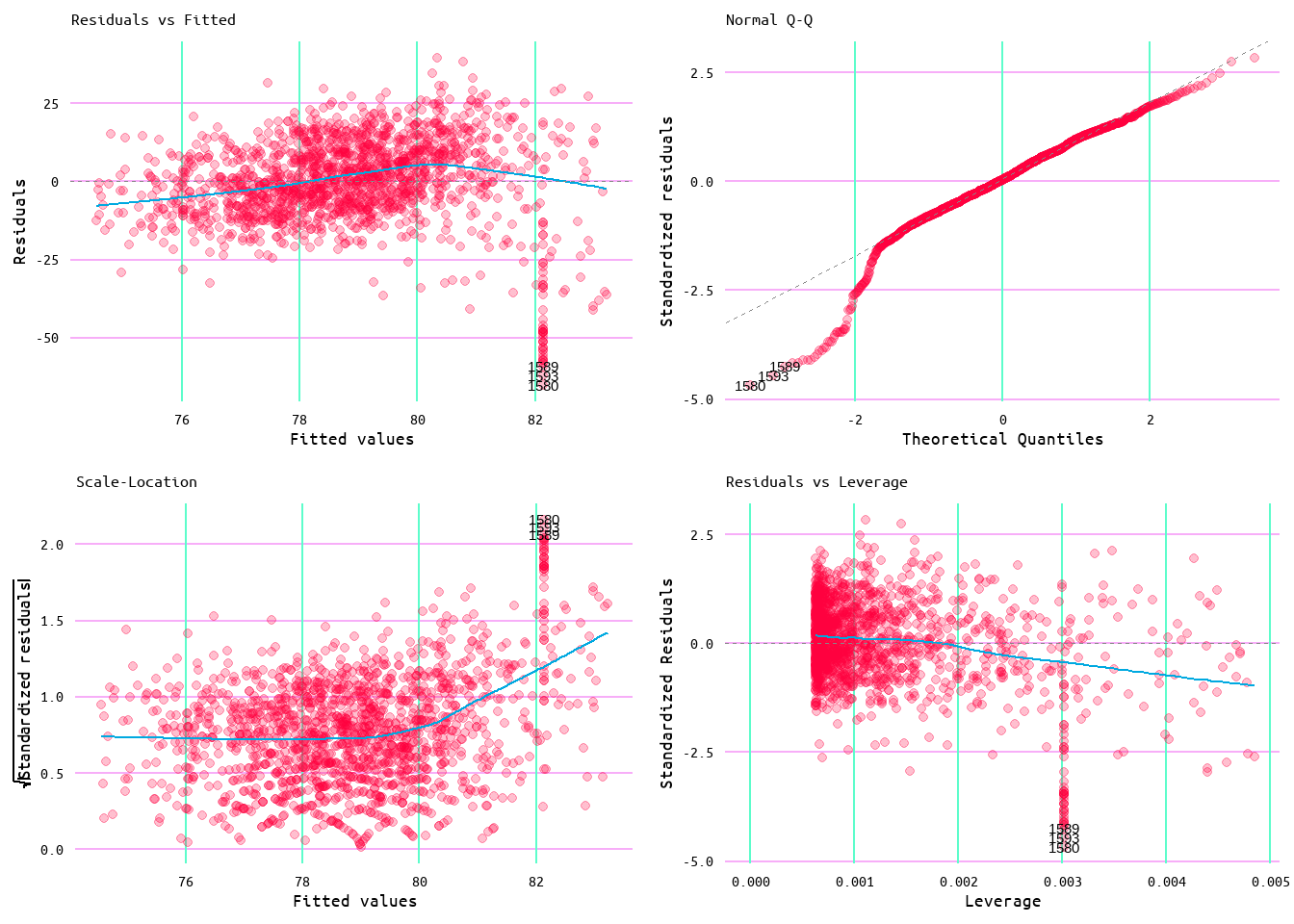
Figure 30: Diagnostic Plots for Losses and Runs Scored Model 2
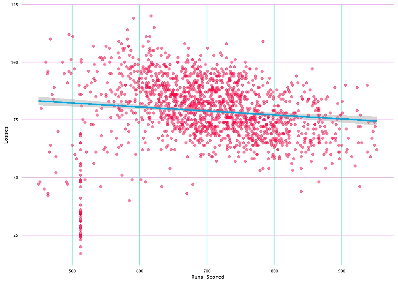
Figure 31: Regression Plot for Losses and Runs Scored Model 2
Losses ~ Runs Allowed Model
Moving from runs scored to runs allowed, the initial model produced an R2 value of 0.39 with a residual standard error of 9.68 (see Table 17). This beats the performance of the wins and runs scored model, which had an original R2 value of 0.35 and residual standard error of 10.03. Looking at Figure 32, the regression plot for this model shows that the relationship between losses and runs allowed is quite linear.
Looking at Figure 33 for the diagnostic plots, similar patterns that appeared in the wins and runs scored model likewise appear here. As such, despite this model generally meeting the assumptions, the same log transformation of the independent (runs allowed) variable that was applied to the wins and runs scored model was applied here. This was mainly done to provide a comparison of the log transformed models, as well to see what improvements could be made to the single-predictor model.
The log transformation of runs allowed returned a very minor improvement as the R2 value remained at 0.39 and the residual standard error stayed approximately the same at 9.65 (see Table 18). The diagnostic plots do show some improvement in terms of meeting the linear regression assumptions (see Figure 34); however, the log transformation only appears to shift the distribution of the values (see Figure 35). Given the minor improvement to the model and the shifting of the distribution, this transformation is not really necessary and using the non-transformed variables would be fine.
| r.squared | adj.r.squared | sigma | statistic | p.value | df | logLik | AIC | BIC | deviance | df.residual | nobs |
|---|---|---|---|---|---|---|---|---|---|---|---|
| 0.51 | 0.51 | 9.81 | 1674.42 | 0 | 1 | -5907.38 | 11820.76 | 11836.89 | 153293.6 | 1594 | 1596 |
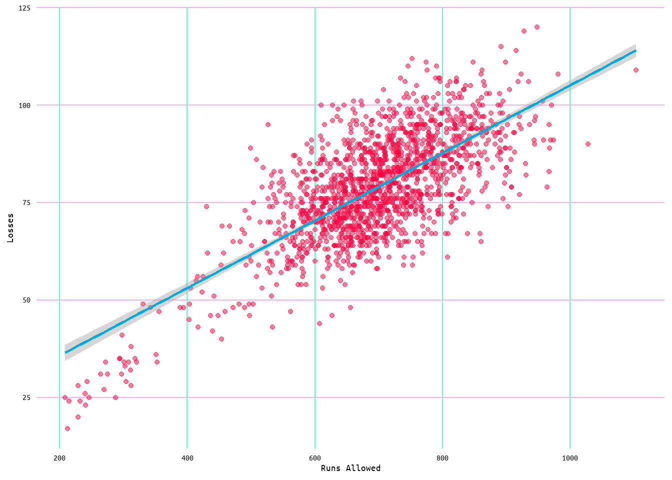
Figure 32: Regression Plot for Losses and Runs Allowed Model 1
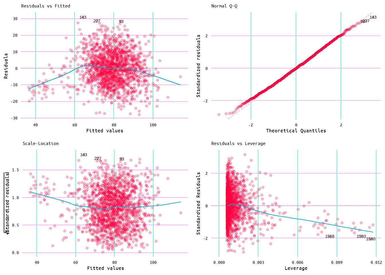
Figure 33: Diagnostic Plots for Losses and Runs Allowed Model 1
| r.squared | adj.r.squared | sigma | statistic | p.value | df | logLik | AIC | BIC | deviance | df.residual | nobs |
|---|---|---|---|---|---|---|---|---|---|---|---|
| 0.53 | 0.53 | 9.59 | 1825.68 | 0 | 1 | -5871.28 | 11748.56 | 11764.69 | 146513.4 | 1594 | 1596 |
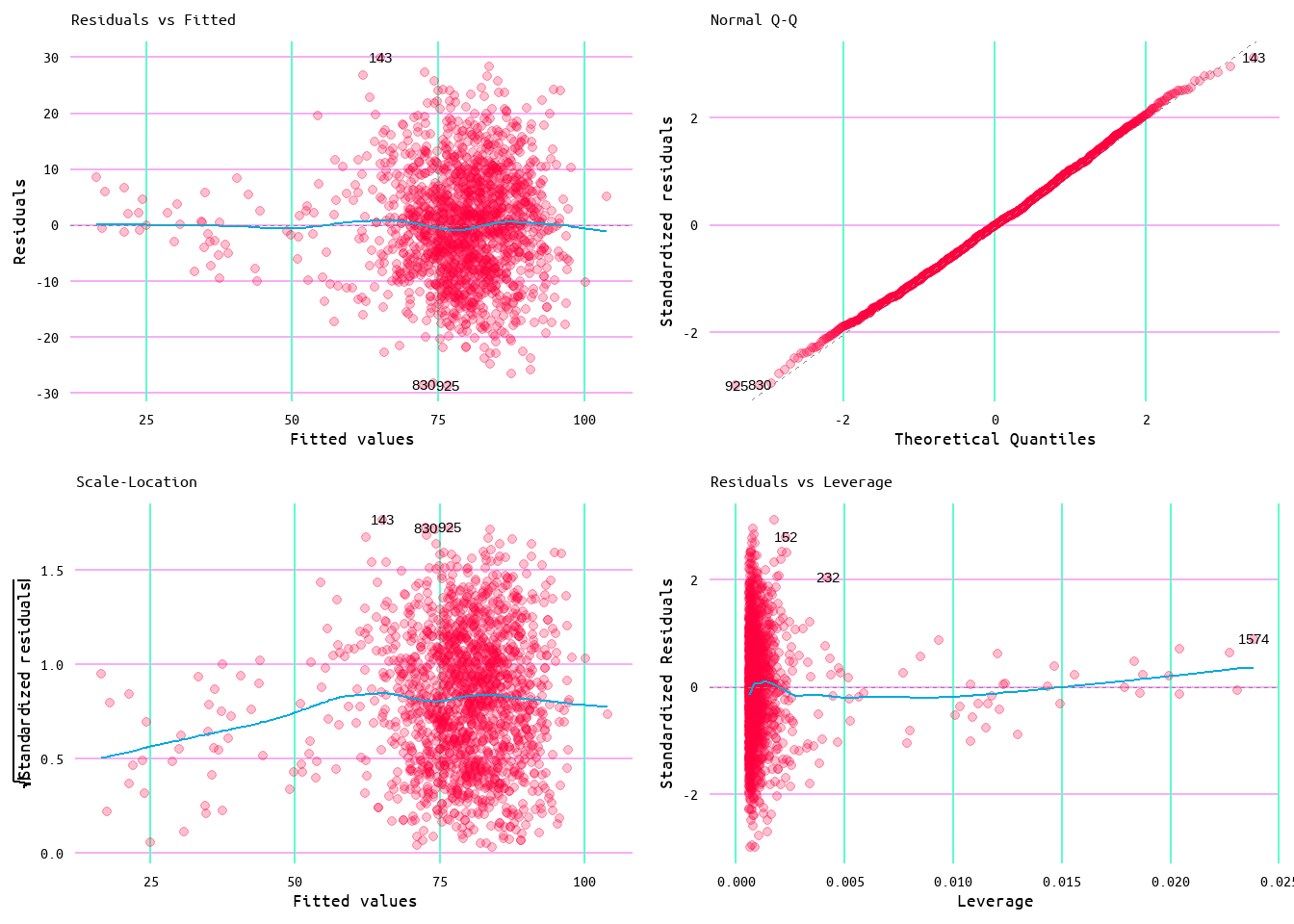
Figure 34: Diagnostic Plots for Losses and Runs Allowed Model 2
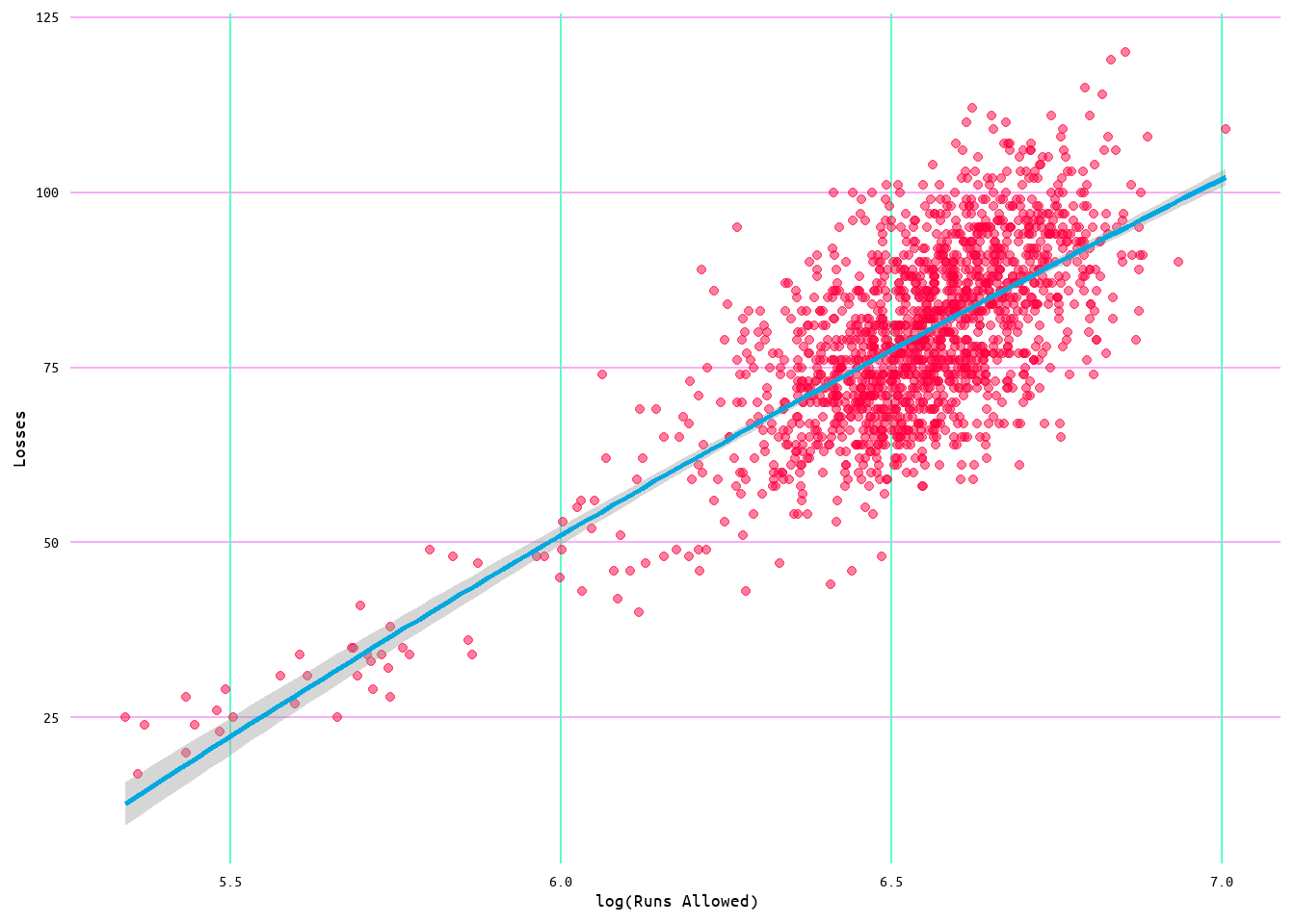
Figure 35: Regression Plot for Losses and Runs Allowed Model 2
Losses ~ Runs Allowed Minus Home Runs Allowed Model
And lastly, losses was also run in a model with runs allowed minus home runs allowed in an attempt to model defense with the influence of pitching weakened. This is again a very basic stand-in for defense without pitching but hey, this is for fun.
The model for this regression returned an R2 value of 0.44 with a residual standard error of 9.27 (see Table 19). Meaning, that with home runs removed, runs allowed accounted for ~44% of the variance in losses with an average error of 9.27. Looking at the regression plot in Figure 36, the relationship between losses and runs allowed minus home runs allowed is quite linear. Which makes sense given the relationship between losses and runs allowed. Moreover, the diagnostic plots for this model, shown in Figure 37, show very similar results as to those for the non-transformed losses and runs allowed model. As the log transformation of runs allowed in the losses and runs allowed model only returned minor improvements regarding the results, I did not find it pertinent to apply the same transformation to this model.
| r.squared | adj.r.squared | sigma | statistic | p.value | df | logLik | AIC | BIC | deviance | df.residual | nobs |
|---|---|---|---|---|---|---|---|---|---|---|---|
| 0.56 | 0.56 | 9.3 | 2039.55 | 0 | 1 | -5822.87 | 11651.74 | 11667.86 | 137889.4 | 1594 | 1596 |
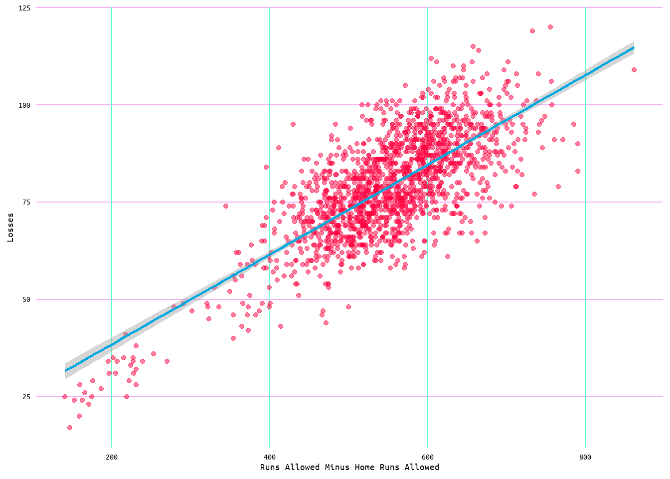
Figure 36: Regression Plot for Losses and Runs Allowed Minus Home Runs Allowed
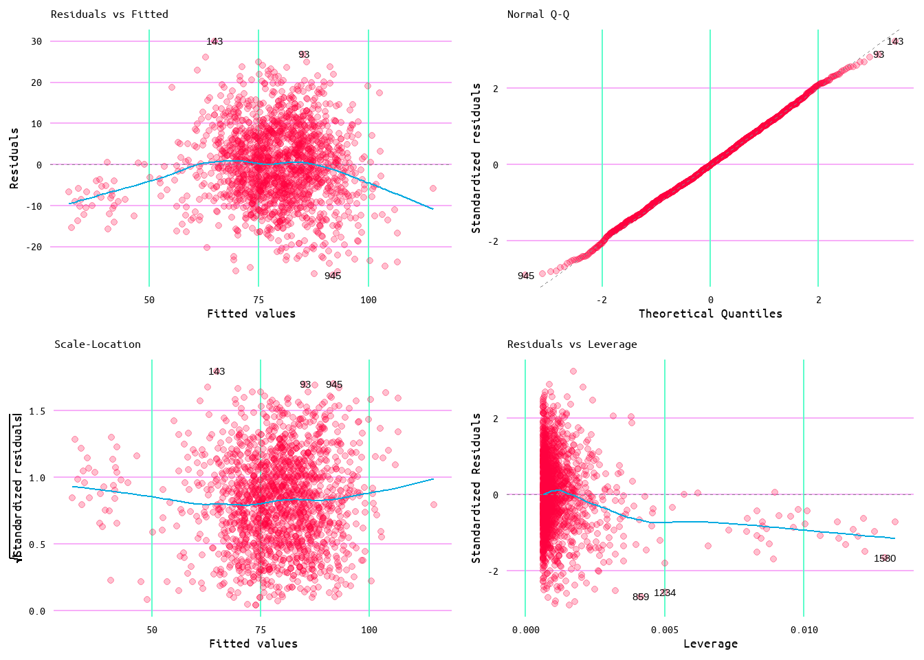
Figure 37: Diagnostic Plots for Losses and Runs Allowed Minus Home Runs Allowed
Discussion
So what does all of this mean?
I was originally inspired to perform this analysis as I was left with questions from the Baseball Prospectus article on defensive metrics. The purpose being to assess whether defense truly was nowhere near as important as hitting or pitching. Originally I was only going to do a simplistic correlation analysis, but I decided to grow that into a linear regression analysis, which in turn led me to diving deeper into subjects of variable transformation, outlier analysis, and visualization.
My idea for analysing the contributions of offense and defense was to model offense as runs scored and defense as runs allowed, with the contributions of both to wins and losses. In an attempt to also account for the influence of pitching in runs allowed, the number of home runs allowed was subtracted from runs allowed. However, this presents as a simple means of accommodating for pitching and does not truly address the involvement of pitching in runs allowed.
To address the contributions of offense and defense, linear regression models were created of both variables with the associated outcome variable (i.e., runs scored and wins and runs allowed and losses) as well as with the opposing outcome variable (i.e., runs scored and losses and runs allowed and wins). The purpose being to see which of runs scored and runs allowed accounts for more variance in the associated outcome variable, as well as which of runs scored and runs allowed better accounts for variance in the opposing variable. While the simplicity of this analysis makes it difficult to draw any strong conclusions from this analysis, the results do suggest that defense is not nowhere near as important as at least offense. In the case of associated outcome variable, runs allowed performs better in terms of accounting for variance in its associated variabled (losses) than does runs scored (wins). Moreover, in both the non-transformed and transformed models, runs allowed performed better in accounting for variance in the opposing outcome variable than did runs scored. As such, as the simplicity of these models do not provide for any strong conclusions, indeed results of the opposing outcome models suggest that the single-predictor is not enough to account for the variance seen, the results do suggest a pattern that points to the importance of defense in baseball. This can be understood as follows: to win a game, a team must score runs; to not lose a game, a team must prevent runs. A team could set a club record for the number of runs scored in a game, yet still lose that game if the other team scores more. Likewise, a team could prevent the other team from ever scoring, yet still not win if they do not score any runs themselves. To say that defense is nowhere near as important as offense is a misnomer, and a statement that I believe comes from the biases born from the difficulty in assessing defensive contributions and the robustness of current offensive metrics.